learning Phrase Representations

Introduction

In this paper, Cho et al. propose a novel neural network model called RNN Encoder–Decoder that consists of two recurrent neural networks (RNN). One RNN encodes a sequence of symbols into a fixed length vector representation, and the other decodes the representation into another sequence of symbols. The encoder and decoder of the proposed model are jointly trained to maximize the conditional probability of a target sequence given a source sequence. The performance of a statistical machine translation system is empirically found to improve by using the conditional probabilities of phrase pairs computed by the RNN Encoder–Decoder as an additional feature in the existing log-linear model.

RNN Encoder–Decoder

In this paper, researchers propose a novel neural network architecture that learns to encode a variable-length sequence into a fixed-length vector representation and to decode a given fixed-length vector representation back into a variable-length sequence. From a probabilistic perspective, this new model is a general method to learn the conditional distribution over a variable-length sequence conditioned on yet another variable-length sequence, e.g. [math]\displaystyle{ p(y_1, . . . , y_{T'} | x_1, . . . , x_T ) }[/math], where one should note that the input and output sequence lengths [math]\displaystyle{ T }[/math] and [math]\displaystyle{ T' }[/math] may differ.

File:encdec1.png

Fig 1. An illustration of the proposed RNN Encoder–Decoder.

The encoder is an RNN that reads each symbol of an input sequence x sequentially. As it reads each symbol, the hidden state of the RNN changes.

[math]\displaystyle{ h_t=f(h_{t-1},x_t) }[/math]

After reading the end of the sequence (marked by an end-of-sequence symbol), the hidden state of the RNN is a summary [math]\displaystyle{ \mathbf{c} }[/math] of the whole input sequence.

The decoder of the proposed model is another RNN which is trained to generate the output sequence by predicting the next symbol [math]\displaystyle{ y_t }[/math] given the hidden state[math]\displaystyle{ h_t }[/math] . However, as shown in figure 1, both [math]\displaystyle{ y_t }[/math] and [math]\displaystyle{ h_t }[/math] are also conditioned on [math]\displaystyle{ y_{t-1} }[/math] and on the summary [math]\displaystyle{ \mathbf{c} }[/math] of the input sequence. Hence, the hidden state of the decoder at time [math]\displaystyle{ t }[/math] is computed by,

[math]\displaystyle{ h_t=f(h_{t-1},y_{t-1},\mathbf{c}) }[/math]

and similarly, the conditional distribution of the next symbol is

[math]\displaystyle{ P(y_t|y_{t-1},y_{t-2},\cdots,y_1,\mathbf{c})=g(h_t,,y_{t-1},\mathbf{c}) }[/math]

The two components of the proposed RNN Encoder–Decoder are jointly trained to maximize the conditional log-likelihood

[math]\displaystyle{ \max_{\mathbf{\theta}}\frac{1}{N}\sum_{n=1}^{N}\log p_\mathbf{\theta}(\mathbf{y}_n|\mathbf{x}_n) }[/math]

where [math]\displaystyle{ \mathbf{\theta} }[/math] is the set of the model parameters and each [math]\displaystyle{ (\mathbf{y}_n,\mathbf{x}_n) }[/math] is an (input sequence, output sequence) pair from the training set. In our case, as the output of the decoder, starting from the input, is differentiable, the model parameters can be estimated by a gradient-based algorithm. Once the RNN Encoder–Decoder is trained, the model can be used in two ways. One way is to use the model to generate a target sequence given an input sequence. On the other hand, the model can be used to score a given pair of input and output sequences.

Hidden Unit that Adaptively Remembers and Forgets

This paper also propose a new type of hidden node that has been inspired by LSTM but is much simpler to compute and implement. Fig. 2 shows the graphical depiction of the proposed hidden unit.

File:encdec2.png

Fig 2. An illustration of the proposed hidden activation function. The update gate z selects whether the hidden state is to be updated with a new hidden state h˜. The reset gate r decides whether the previous hidden state is ignored.

Mathematically it can be shown as([math]\displaystyle{ \sigma }[/math] is the logistic sigmoid function, [math]\displaystyle{ [.]_j }[/math] denotes the j-th element of a vector and [math]\displaystyle{ \odot }[/math] means elementwise multiply):

[math]\displaystyle{ r_j=\sigma([\mathbf{W}_r\mathbf{x}]_j+[\mathbf{U}_r\mathbf{h}_{t-1}]_j ) }[/math]

[math]\displaystyle{ z_j=\sigma([\mathbf{W}_z\mathbf{x}]_j+[\mathbf{U}_z\mathbf{h}_{t-1}]_j ) }[/math]

[math]\displaystyle{ h_j^{(t)}=z_jh_j^{(t-1)}+(1-z_j)\tilde{h}_j^{(t)} }[/math]

where

[math]\displaystyle{ \tilde{h}_j^{(t)}=\phi([\mathbf{W}\mathbf{x}]_j+[\mathbf{U}(\mathbf{r}\odot\mathbf{h}_{t-1})]_j ) }[/math]

In this formulation, when the reset gate is close to 0, the hidden state is forced to ignore the previous hidden state and reset with the current input only. This effectively allows the hidden state to drop any information that is found to be irrelevant later in the future, thus, allowing a more compact representation. On the other hand, the update gate controls how much information from the previous hidden state will carry over to the current hidden state. This acts similarly to the memory cell in the LSTM network and helps the RNN to remember longterm information. Furthermore, this may be considered an adaptive variant of a leaky-integration unit.<ref> Bengio Y, Boulanger-Lewandowski N, Pascanu R. Advances in optimizing recurrent networks[C]//Acoustics, Speech and Signal Processing (ICASSP), 2013 IEEE International Conference on. IEEE, 2013: 8624-8628. </ref>

Because each hidden unit has separate gates, it is possible for each hidden to unit to learn to capture dependencies over different lengths of time (determined by the frequency at which its reset and updates gates are active).

Scoring Phrase Pairs with RNN Encoder–Decoder

In a commonly used statistical machine translation system (SMT), the goal of the system (decoder, specifically) is to find a translation f given a source sentence e, which maximizes

[math]\displaystyle{ p(\mathbf{f} | \mathbf{e})\propto p(\mathbf{e} | \mathbf{f})p(\mathbf{f}) }[/math]

where the first term at the right hand side is called translation model and the latter language model (see, e.g., (Koehn, 2005)). In practice, however, most SMT systems model [math]\displaystyle{ \log p(\mathbf{f} | \mathbf{e}) }[/math] as a loglinear model with additional features and corresponding weights:

[math]\displaystyle{ \log p(\mathbf{f} | \mathbf{e})=\sum_{n=1}^Nw_nf_n(\mathbf{f},\mathbf{e})+\log Z(\mathbf{e}) }[/math]

where [math]\displaystyle{ f_n }[/math] and [math]\displaystyle{ w_n }[/math] are the n-th feature and weight, respectively. [math]\displaystyle{ Z(\mathbf{e}) }[/math] is a normalization constant that does not depend on the weights. The weights are often optimized to maximize the BLEU score on a development set.

Cho et al. propose to train the RNN Encoder–Decoder on a table of phrase pairs and use its scores as additional features in the loglinear model showed above when tuning the SMT decoder. For training the RNN-Encoder-Decoder, phrase frequency is ignored for several reasons: to reduce computation time, to ensure the model does not simply rank phrases by frequency, and because frequency information is already encoded in the features for the SMT (so it's better to not use the capacity of the RNN-Encoder-Decoder redundantly).

Experiments

The model is evaluated on the English/French translation task of the WMT’14 workshop. In building the model Cho et al. used baseline phrase-based SMT system and a Neural Language Model(CSLM)<ref> Schwenk H, Costa-Jussa M R, Fonollosa J A R. Continuous space language models for the IWSLT 2006 task[C]//IWSLT. 2006: 166-173. </ref>

They tried the following combinations: 1. Baseline configuration 2. Baseline + RNN 3. Baseline + CSLM + RNN 4. Baseline + CSLM + RNN + Word penalty

Results:

File:encdec3.png

Fig 3. BLEU scores computed on the development and test sets using different combinations of approaches. WP denotes a word penalty, where we penalizes the number of unknown words to neural networks.

The best performance was achieved when we used both CSLM and the phrase scores from the RNN Encoder–Decoder. This suggests that the contributions of the CSLM and the RNN Encoder– Decoder are not too correlated and that one can expect better results by improving each method independently

Word and Phrase Representations

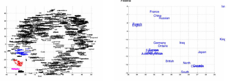
As the presented model maps sentences into a continuous space vector and prior continuous space language models have been known to learn semantically meaningful embeddings, one could expect this to happen for the presented model, too. This is indeed the case. When projecting to a 2D space (with Barnes-Hut-SNE), semantically similar words are clearly clustered.

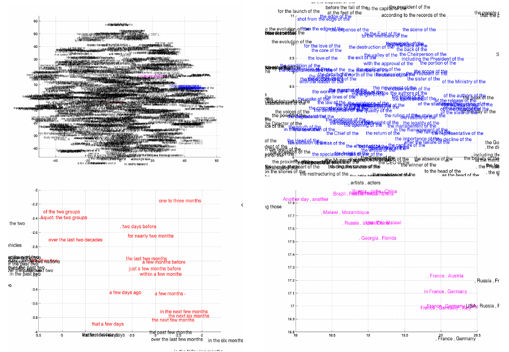
Phrases are also clustered capturing both semantic and syntactic structures.

References

<references />