goingDeeperWithConvolutions

Introduction

In the last three years, due to the advances of deep learning and more concretely convolutional networks [an introduction of CNN] , the quality of image recognition has increased dramatically. The error rates for ILSVRC competition dropped significantly year-by-year [LSVRC]. This paper<ref name=gl> Szegedy, Christian, et al. "Going deeper with convolutions." arXiv preprint arXiv:1409.4842 (2014). </ref> propose a new deep convolutional neural network architecture code-named Inception. With the Inception module and carefully-crafted design, researchers build a 22 layers deep network called Google Lenet, which uses 12 times less parameters while being significantly more accurate than the winners of ILSVRC 2012.<ref name=im> Krizhevsky, Alex, Ilya Sutskever, and Geoffrey E. Hinton. "Imagenet classification with deep convolutional neural networks."

Advances in neural information processing systems. 2012.

</ref>

Motivation

The authors main motivation for their "Inception module" approach to CNN architecture is due to:

• Large CNN networks may allow for more expressive power, however it is also prone to over fitting due to the large number of parameters.
• Uniform increased network size increases computational resources.
• Sparse networks are theoretically possible, but sparse data structures are very inefficient.

Why Sparse Matrices are inefficient

Sparse matrices if stored as Compressed Row Storage (CSR) format or any other common sparse matrix data structures can be expensive to access at specific indices of the matrix. This is because they use an indirect addressing step for every single scalar operation in a matrix-vector product. (source: netlib.org manual) Because of this indirection the values are not stored in one contiguous memory location and a lot of cache misses occur which slow down the calculation as data has to be fetched from the slower main memory.

For example a non-symmetric sparse matrix A in CRS format defined by:

File:crs sparse matrix.gif

The CRS format for this matrix is then specified by arrays `{val, col_ind, row_ptr}` given below:

File:crs sparse matrix details 1.gif

File:crs sparse matrix details 2.gif

Background

The paper assumes that the reader is familiar with Convolutional Neural Networks (CNNs). This section gives a short introduction based on this tutorial.

In a CNN the layers are sparsely connected. Each unit in layer [math]\displaystyle{ m }[/math] receives only inputs from part of layer [math]\displaystyle{ m-1 }[/math]. This inputs are usually from spatially neighboring units and the connection weights to each unit in layer [math]\displaystyle{ m }[/math] are shared. This reduces the amount of computation (because the layers are not fully connected) and reduces the amount of parameters to learn so that less training data is required and the network is less prone to overfitting. Because this structure is similar to a convolution in the sense that the same set of weights get shifted over the input and applied at each location, networks with this structure are called convolutional neural networks.

A related approach is max-pooling. Instead of weighting the input values and summing them, as in a standard artificial neural network, the maximum value out of the max-pooling window in picked. By picking one value out of [math]\displaystyle{ n \times n }[/math] ([math]\displaystyle{ 3 \times 3 = 9 }[/math] in the paper) the amount of computation for the higher layer gets reduced. Furthermore, a form of translation invariance is provided because shifting the max-pooling window by one position will likely still give the same maximum.

Related work

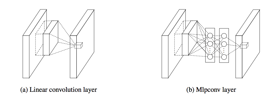
In 2013 Lin et al.<ref name=nin> Min Lin, Qiang Chen and Shuicheng Yan. Network in Network </ref> pointed out that the convolution filter in CNN is a generalized linear model (GLM) for the underlying data patch and the level of abstraction is low with GLM. They suggested replacing GLM with a ”micro network” structure which is a general nonlinear function approximator.

Fig 1. Comparison of linear convolution layer and mlpconv layer

Also in this paper<ref name=nin></ref> Lin et al. proposed a new output layer to improve the performance. In tradition the feature maps of the last convolutional layers are vectorized and fed into a fully connected layers followed by a softmax logistic regression layer<ref name=im></ref>. Lin et al. argued that this structure is prone to overfitting, thus hampering the generalization ability of the overall network. To improve this they proposed another strategy called global average pooling. The idea is to generate one feature map for each corresponding category of the classification task in the last mlpconv layer, take the average of each feature map, and the resulting vector is fed directly into the softmax layer. Lin et al. claim that their strategy has the following advantages over fully connected layers. First, it is more native to the convolution structure by enforcing correspondences between feature maps and categories. Thus the feature maps can be easily interpreted as categories confidence maps. Second, there is no parameter to optimize in the global average pooling thus overfitting is avoided at this layer. Furthermore, global average pooling sums out the spatial information, thus it is more robust to spatial translations of the input.

Inception module

The Inception architecture in "Going deeper with convolutions", Szegedy, Christian, et al. is based on two main ideas: The approximation of a sparse structure with spatially repeated dense components and using dimension reduction to keep the computational complexity in bounds, but only when required.

Convolutional filters with different sizes can cover different clusters of information. By finding the optimal local construction and repeating it spatially (assuming translational invariance), they approximate the optimal sparse structure with dense components. For convenience of computation, they choose to use 1 x 1, 3 x 3 and 5 x 5 filters. Additionally, since pooling operations have been essential for the success in other state of the art convolutional networks, they also add pooling layers in their module. Together these made up the naive Inception module.

File:i1.png

Fig 2. Inception module, naive version

Stacking these inception modules on top of each would lead to an exploding number of outputs. Thus, they use, inspired by "Network in Network", Szegedy, Christian, et al., 1x1 convolutions for dimensionality reduction. While this keeps the computational complexity in bounds, it comes with another problem. The low dimensional embeddings represent the data in a compressed and non-sparse form, but the first idea requires sparsity to make the approximation possible. For that reason, the dimensionality reduction step should only be applied when it is required to preserve sparse representations as much as possible. In practice, the author's used the 1x1 convolutions before doing the expensive 3 x 3 and 5 x 5 convolutions.

File:i2.png

Fig 3. Inception module with dimension reduction

Beneficial aspects of Inception module

• It allows for increasing number of units significantly without an uncontrolled blow-up in computational complexity.
• The ubiquitous use of dimension reduction allows for shielding the large number of input filters of the last stage to the next layer.
• It aligns with the intuition that visual information should be processed at various scales and then aggregated so that the next stage can abstract features from different scales simultaneously.
• It can result in networks that are 2-3X faster than similarly performing networks with non-inception architecture.

Google Lenet

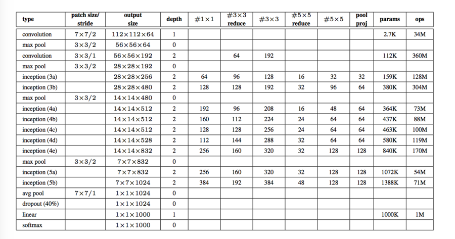
The structure of Google Lenet can be seen from this figure.

“#3 x 3 reduce” and “#5 x 5 reduce” stands for the number of 1 x 1 filters in the reduction layer used before the 3 x 3 and 5 x 5 convolutions.

In order to encourage discrimination in the lower stages in the classifier and increase the gradient signal that gets propagated back, the authors add auxiliary classifiers connected to the out put of (4a) and (4d). During training, their loss gets added to the total loss of the network with a discount weight (the losses of the auxiliary classifiers were weighted by 0.3). At inference time, these auxiliary networks are discarded.

The networks were trained using the DistBelief<ref> Dean, Jeffrey, et al. "Large scale distributed deep networks." Advances in Neural Information Processing Systems. 2012. </ref> distributed machine learning system using modest amount of model and data-parallelism.

ILSVRC 2014 Classification Challenge Results

The ILSVRC 2014 classification challenge involves the task of classifying the image into one of 1000 leaf-node categories in the Imagenet hierarchy ILSVRC. In calculating the error rate for the table below, an image was considered to be correctly classified if its true class was among the top 5 predicted classes.

Szegedy, Christian, et al. independently trained 7 versions of the same GoogLeNet model (they only differ in sampling methodologies and the random order in which they see input images), and performed ensemble prediction with them.

Team	Year	Place	Error (top-5)	Uses external data
SuperVision	2012	1st	16.4%	no
SuperVision	2012	1st	15.3%	Imagenet 22k
Clarifi	2013	1st	11.7%	no
Clarifi	2013	1st	11.2%	Imagenet 22k
MSRA	2014	3rd	7.35%	no
VGG	2014	2nd	7.32%	no
GoogleLeNet	2014	1st	6.67%	no

Critques

• It is quite interesting how the authors of this paper tried to address computational efficiency by condensing the network into a more dense form. What the paper perhaps did not mention is whether this computationally efficient dense network has any robustness trade-off. Additionally, it is a bit paradoxical to say that a large network with many parameters may induce over training, while intuitively correct, conversely techniques such as Dropout <ref>Srivastava, Nitish, et al. "Dropout: A simple way to prevent neural networks from overfitting." The Journal of Machine Learning Research 15.1 (2014): 1929-1958.</ref> encourage a sparse network representation to avoid over training and increase robustness. Further study is needed to investigate whether one should approach CNN training in a dense, sparse, or happy medium between two architecture types.

References

<references />