measuring statistical dependence with Hilbert-Schmidt norms

This is another very popular kernel-based approach fro detecting dependence which is called HSIC(Hilbert-Schmidt Independence Criteria). It's based on the eigenspectrum of covariance operators in reproducing kernel Hilbert spaces(RKHSs).This approach is simple and no user-defined regularisation is needed. Exponential convergence is guaranteed, so convergence is fast.

Background

Before the proposal of HSIC, there are already a few kernel-based independence detecting methods. Bach[] proposed a regularised correlation operator which is derived from the covariance and cross-covariance operators, and its largest singular value was used as a static to test independence. Gretton et al.[] used the largest singular value of the cross-covariance operator which resulted constrained covariance(COCO). HSIC is a extension of the concept COCO by using the entire spectrum of cross-covariance operator to determine when all its singular values are zero rather than just looking the largest singular value. The HSIC resolves the question regarding the link between the quadratic dependence measure and kernel dependence measures based on RKHSs, and generalizes the measure to metric spaces.

Cross-Covariance Operators

Hilbert-Schmidt Norm. Denote by [math]\displaystyle{ \mathit{C}:\mathcal{G}\to\mathcal{F} }[/math] a linear operator. Provided the sum converges, the HS norm of [math]\displaystyle{ \mathit{C} }[/math] is defined as

[math]\displaystyle{ ||\mathit{C}||^2_{HS}:=\sum_{i,j}\lt \mathit{C}v_i,u_j\gt _\mathcal{F}^2 }[/math]

Where [math]\displaystyle{ v_i,u_j }[/math] are orthonormal bases of [math]\displaystyle{ \mathcal{G} }[/math] and [math]\displaystyle{ \mathcal{F} }[/math] respectively.

Hilbert-Schmidt Operator is defined based on the definition of Hilbert Schmidt norm as

[math]\displaystyle{ \lt \mathit{C},\mathit{D}\gt {HS}:=\sum_{i,j}\lt \mathit{C}v_i,u_j\gt _\mathcal{F}\lt \mathit{D}v_i,u_j\gt _\mathcal{F} }[/math]

Tensor Product. Let [math]\displaystyle{ f\in \mathcal{F} }[/math] and [math]\displaystyle{ g\in \mathcal{G} }[/math]. The tensor product operator [math]\displaystyle{ f\otimes g:\mathcal{G}\to \mathcal{F} }[/math] is defined as

[math]\displaystyle{ (f\otimes g)h:=f\lt g,h\gt _\mathcal{G} }[/math] for all [math]\displaystyle{ h\in \mathcal{G} }[/math]

Cross-Covariance Operator associated with the joint measure [math]\displaystyle{ p_{x,y} }[/math] on [math]\displaystyle{ (\mathcal{X}\times\mathcal{Y},\Gamma\times\Lambda) }[/math] is a linear operator [math]\displaystyle{ C_{xy}:\mathcal{G}\to \mathcal{F} }[/math] defined as

[math]\displaystyle{ C_{xy}:=E_{x,y}[(\theta (x)-\mu_x)\otimes (\psi (y)-\mu_y)]=E_{x,y}[\theta (x)\otimes \psi (y)]-\mu_x\otimes\mu_y }[/math]

Hilbert-Schmidt Independence Criterion

Given separable RKHSs [math]\displaystyle{ \mathcal{F},\mathcal{G} }[/math] and a joint measure [math]\displaystyle{ p_{xy} }[/math] over [math]\displaystyle{ (\mathcal{X}\times\mathcal{Y},\Gamma\times\Lambda) }[/math], HSIC is defined as the squared HS-norm of the associated cross-covariance operator [math]\displaystyle{ C_{xy} }[/math]:

[math]\displaystyle{ HSIC(p_{xy},\mathcal{F},\mathcal{G}):=||C_{xy}||_{HS}^2 }[/math]

According to Gretton et al., the largest singular value [math]\displaystyle{ ||C_{xy}||_{HS}=0 }[/math] if and only if x and y are independent. Since [math]\displaystyle{ ||C_{xy}=0||_S }[/math] if and only if [math]\displaystyle{ ||C_{xy}||_{HS}=0 }[/math], so [math]\displaystyle{ ||C_{xy}||_{HS}=0 }[/math] if and only if x and y are independent. Therefore, HSIC can be used as a independence criteria.

Estimator of HSIC

Let [math]\displaystyle{ Z:={(x_1,y_1),\dots,(x_m,y_m)}\subseteq \mathcal{X}\times\mathcal{Y} }[/math] be a series of m independent observations drawn from [math]\displaystyle{ p_{xy} }[/math]. An empirical estimator of HSIC, written HSIC(Z,\mathcal{F},\mathcal{G}) is given by

[math]\displaystyle{ HSIC(Z,\mathcal{F},\mathcal{G}):=(m-1)^{-2}trKHLH }[/math]

where [math]\displaystyle{ H,K,L\in \mathbb{R}^{m\times m},K_{ij}:=k(x_i,x_j),L_{i,j}:=l(y_i,y_j) and H_{ij}:=\delta_{ij}-m^{-1} }[/math]. It can be proved that the bias of the empirical HSIC is at [math]\displaystyle{ \mathit{O}(m^{-1}) }[/math]. It can be further shown that the deviation between [math]\displaystyle{ HSIC(Z,\mathcal{F},\mathcal{G}) }[/math] and its expectation is not too large.

Independence Tests

Demixing of n randomly chosen i.i.d. samples of length m, where n varies from 2 to 16. The Gaussian kernel results are denoted g, and the Laplace kernel results l. The column Rep. gives the number of runs over which the average performance was measured. Note that some algorithm names are truncated: Fica is Fast ICA, IMAX is Infomax, RAD is RADICAL, CFIC is CFICA, CO is COCO, and HS is HSIC. Performance is measured using the Amari divergence (smaller is bettter).

File:hsic table1.png

In the experiment, HSIC with a Gaussian kernel performs on par with the best alternatives in the final four experiments, and that HSIC with a Laplace kernel gives joint best performance in six of the seven experiments. On the other hand, RADICAL and the KGV perform better than HSIC in the m = 250 case.

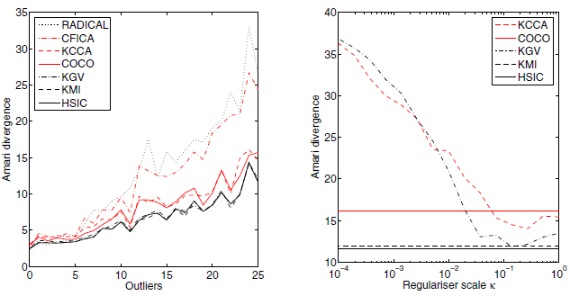
Left: Effect of outliers on the performance of the ICA algorithms. Each point represents an average Amari divergence over 100 independent experiments (smaller is better). The number of corrupted observations in both signals is given on the horizontal axis. Right: Performance of the KCC and KGV as a function of κ for two sources of size m = 1000, where 25 outliers were added to each source following the mixing procedure.

HSIC is much more robust to outliers in comparing to other methods. This method doesn't need regularisation, while KGV and KCC is sensitive to regulariser scale.

Summary

By using the HS norm of the cross-covariance, HSIC is simpler to define, requires no regularisation or tuning beyond kernel selection. It's robust to noise and efficient compared to other methods. The performance meets or exceeds the best alternative on all data sets besides the m=250 case.

References

[1] Gretton, Arthur, et al. "Measuring statistical dependence with Hilbert-Schmidt norms." Algorithmic learning theory. Springer Berlin Heidelberg, 2005.

[2] Fukumizu, Kenji, Francis R. Bach, and Michael I. Jordan. "Kernel dimension reduction in regression." The Annals of Statistics 37.4 (2009): 1871-1905.

[3] Bach, Francis R., and Michael I. Jordan. "Kernel independent component analysis." The Journal of Machine Learning Research 3 (2003): 1-48.

[4] Baker, Charles R. "Joint measures and cross-covariance operators." Transactions of the American Mathematical Society 186 (1973): 273-289.