video-based face recognition using Adaptive HMM

\draft

Introduction

Human face recognition

Human face recognition is a subarea of object recognition aims to identify persons face given a scene or still images. Face recognition benefits many fields such as computer security and video compression. Two approaches are commonly used in face recognition are video-based and still images. Since 80’s, image-based recognition approach is more dominant in face recognition in comparison with the video-based approach. Few recent studies took advantages of the features of video scenes as it provides more dynamic characteristic of the human face that help the recognition process. Also, video scene provides more features of 3D representation and high resolution images. Besides, in video-based recognition the prediction accuracy can be improved using the farm sequence. Motivated by speaker adaptation, this paper presents an Adaptive Hidden Markov model to recognise human face from frames sequence. The proposed model train HMM on the training data and then improve the recognition constantly using the test data.

Hidden Markov Model (HMM)

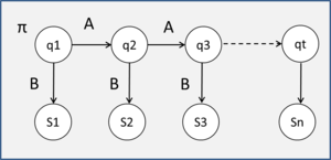
Hidden Markov Model is graphical model that suitable to represent sequential data. HMM consists of the probability of initial state [math]\displaystyle{ \pi_i }[/math], unobserved states [math]\displaystyle{ q_t }[/math], the probability of transition matrix A, and emission matrix B. HMM characterized by [math]\displaystyle{ \lambda=(A,B,\pi) }[/math] :

Fig.1 HMM graph.

Given N of states [math]\displaystyle{ S ={S_1 ,S_2 , ,S_N } }[/math] and [math]\displaystyle{ q_t }[/math] state of time T

A a transition matrix where [math]\displaystyle{ a_ij }[/math] is the (i,j) entry in A:

[math]\displaystyle{ a_ij=P(q_t=S_j|q_{t-1}=S_i) }[/math] where [math]\displaystyle{ 1\leq i,j \leq N }[/math]

B the observation pdf [math]\displaystyle{ B={b_i(O)} }[/math]

[math]\displaystyle{ b_i(O)=\sum_{k=1}^M c_{ik} N(O,\mu_{ik},U_{ik}) }[/math] where [math]\displaystyle{ 1\leq i \leq N }[/math]

where [math]\displaystyle{ c_{ik} }[/math] is the mixture coefficient for [math]\displaystyle{ k_th }[/math] mixure component of [math]\displaystyle{ S_i }[/math]

M number of component in Gaussian mixture model .

[math]\displaystyle{ \mu_{ik} }[/math] is the mean vector and [math]\displaystyle{ U_ik }[/math] is the covariance matrix .

the intial state [math]\displaystyle{ \pi_i=p(q_t=S_i) }[/math] wherer [math]\displaystyle{ 1\leq i \leq N }[/math]

Features extraction

In computer vision there is common approaches that in used for features extraction such as Pixel value ,Eigen-coefficients,and DCT. . In this study Principal Component Analysis PCA were used to represent the images in low-dimensional features. The Eigenanalysis was performed to produce new features vectors projected in the eigenspace by computing the covariance, eigenvectors and eigenvalues. The Feature extraction procedure was applied on each on T number of images for each L subjects to generates corresponding feature vectors [math]\displaystyle{ e_{l,t} }[/math]. For all the features vectors the mean vector [math]\displaystyle{ \mu }[/math] and the covariance matrix [math]\displaystyle{ C_e }[/math] were computed.

[math]\displaystyle{ F_l }[/math]={[math]\displaystyle{ f_{l,1},f_{1,2},f_{l,3},……f_{l,t} }[/math]}

[math]\displaystyle{ O_l }[/math]={[math]\displaystyle{ e_{l,1},e_{1,2},e_{l,3},……e_{l,t} }[/math]}

Temporal HMM

Each subject l modeled by fully connected HMM consisted of N states and observed variables O. The training started by intilaizing the HMM [math]\displaystyle{ \lambda=(A,B,\pi) }[/math]. Then the observation vectors are separated using vector quantization into N classes which then used to initially estimate of the probability density function B. Then the MLE [math]\displaystyle{ P(O|\lambda) }[/math]was iteratively computed using EM algorithm as define below:

The probability of initial state is [math]\displaystyle{ \pi_i=\frac{P(O,q_1=i|\lambda)}{P(O|\lambda)} }[/math]

The transition matrix [math]\displaystyle{ a{ij}=\frac {\sum_{t=1}^T P(O,q_{t-1}=i, q_{t}=j|\lambda)}{\sum_{t=1}^T P(O,q_{t-1}=i|\lambda)} }[/math]

The mixture coefficient [math]\displaystyle{ c{ik}=\frac {\sum_{t=1}^T P(q_{t}=i, m_{q,t}=k|O,\lambda)}{\sum_{t=1}^T \sum{k=1}^M P(q_{t}=i,m_{q,t}=k|O,\lambda)} }[/math]

The mean vector [math]\displaystyle{ \mu{ij}=\frac {O_t\sum_{t=1}^T P(q_{t}=i, m_{qt}=k|O,\lambda)}{\sum_{t=1}^T P(q_{t}=i,m_{qt}=k|O,\lambda)} }[/math]

The covariance [math]\displaystyle{ U{ik}=(1-\alpha)C_e+\alpha\frac {\sum_{t=1}^T (O_t-\mu_{ik})(O_t-\mu{it})^T P(q_{t}=i, m_{qt}=k|O,\lambda)}{\sum_{t=1}^T P(q_{t}=i,m_{q,t}=k|O,\lambda)} }[/math]

[math]\displaystyle{ P(O|\lambda_k)=max_l P(o|\lambda_l) }[/math]

Model Evaluation

The proposed model was tested on 3 datasets: Task, Task-new,and Mobo[1].Task database is consisted of videos of 21 subjects while they reading and typing on the computer while the new task datasets contain video of 11 subject in different lighting and cameras settings. Mobo data consisted of 24 video for each subjects while they are in different walking positions. The video frames were cropped manually to 16x16 pixels in Task database and to 48x48 pixels for Mobo database. For each subject, 150 frames were used to for training and 150 for testing. The frames’ location and length were randomly chosen from each user video. To evaluate the performance of the proposed model, the model was compared with a baseline image-recognition algorithm and with the temporal HMM .

The baseline algorithm

The baseline algorithm in this study is individual PCA (IPCA )a commonly used in imaged-based face recognition algorithm recognition Applying the baseline algorithm on Task database yielded a 9.9% error rate with 12 eigenvectors. In Mobo dataset , the baseline algorithm recognition yielded 2.4% error rate using 7 eigenvectors.

Adaptive HMM

The HMM model of Task database consisted of 45 eigenvectors and 12 states for each subjects. The temporal HMM yielded an error rate of 7.0% and the adaptive HMM yielded 4.0% error recognition rate. Temporal HMM and adaptive HMM yielded an error rate of 1.6%, 1.2%, respectively using 30 eigenvectors and 12 HMM states. The results of the evaluation shows that the proposed model outperforms the image-based algorithm as it use more dynamic and temporal features and The adaptive approach enhances the model by using the new observed features in the test sets. Also, IPCA are based on the assumption of single Gaussian distribution while the proposed model based on the assumption of mixture of Gaussian which model the observation better.