stat341f11

Sampling - Sept 20, 2011

The meaning of sampling is to generate data points or numbers such that these data follow a certain distribution.
i.e. From [math]\displaystyle{ x \sim~f(x) }[/math] sample [math]\displaystyle{ \,x_{1}, x_{2}, ..., x_{1000} }[/math]

In practice, it maybe difficult to find the joint distribution of random variables. Through simulating the random variables, we can inference from the data.

Sampling from uniform distribution.

Computers can't generate random numbers as they are deterministic, but they can produce pseudo random numbers. Pseudo random numbers are numbers that mimic the properties of random numbers, but are generated using algorithms. Therefore, they are not truly random.

Multiplicative Congruential

• involves three parameters: integers [math]\displaystyle{ \,a, b, m }[/math], and an initial value [math]\displaystyle{ \,x_0 }[/math] we call the seed
• a sequence of integers is defined as

[math]\displaystyle{ x_{k+1} \equiv (ax_{k} + b) \mod{m} }[/math]

Example: [math]\displaystyle{ \,a=13, b=0, m=31, x_0=1 }[/math] creates a uniform histogram.

MATLAB code for generating 1000 random numbers using the multiplicative congruential method:

a=13;
b=0;
m=31;
x(1)=1;

for ii = 1:1000
    x(ii+1) = mod(a*x(ii)+b,m);
end

MATLAB code for displaying the values of x generated:

x

MATLAB code for plotting the histogram of x:

hist(x)

Facts about this algorithm:

• In this example, the first 30 terms in the sequence are a permutation of integers from 1 to 30 and then the sequence repeats itself.
• Values are between 0 and [math]\displaystyle{ m-1 }[/math], inclusive.
• Dividing the numbers by [math]\displaystyle{ m-1 }[/math] yields numbers in the interval [math]\displaystyle{ [0,1] }[/math].
• MATLAB's rand function once used this algorithm with [math]\displaystyle{ a = 7^5, b = 0, m = 2^{31}-1 }[/math], for reasons described in Park and Miller's 1988 paper "Random Number Generators: Good Ones are Hard to Find" (available online).
• Visual Basic's RND function also used this algorithm with [math]\displaystyle{ a = 1140671485, b = 12820163, m = 2^{24} }[/math] (Reference)

Inverse Transform Method

This is a basic method for sampling. Theoretically using this method we can generate sample numbers at random from any probability distribution once we know its cumulative distribution function (cdf).

Theorem

Take [math]\displaystyle{ U \sim~ \mathrm{Unif}[0, 1] }[/math] and let [math]\displaystyle{ X=F^{-1}(U) }[/math]. Then X has distribution function [math]\displaystyle{ F(\cdot) }[/math], where [math]\displaystyle{ F(x)=P(X \leq x) }[/math].

Let [math]\displaystyle{ F^{-1}( ) }[/math] denote the inverse of [math]\displaystyle{ F( ) }[/math]. Therefore [math]\displaystyle{ F(x)=u \implies x=F^{-1}(u) }[/math]

Proof

Recall that

[math]\displaystyle{ P(a \leq X\lt b)=\int_a^{b} f(x) dx }[/math]

[math]\displaystyle{ cdf=F(x)=P(X \leq x)=\int_{-\infty}^{x} f(x) dx }[/math]

Note that if [math]\displaystyle{ U \sim~ \mathrm{Unif}[0, 1] }[/math], we have [math]\displaystyle{ P(U \leq a)=a }[/math]

[math]\displaystyle{ \begin{align} P(F^{-1}(U) \leq x) &{}= P(F(F^{-1}(U)) \leq F(x)) \\ &{}= P(U \leq F(x)) \\ &{}= F(x) \end{align} }[/math]

Completing the proof.

Continuous Case

Generally it takes two steps to get random numbers using this method.

• Step 1. Draw [math]\displaystyle{ U \sim~ \mathrm{Unif}[0, 1] }[/math]
• Step 2. [math]\displaystyle{ X=F^{-1}(U) }[/math]

Example

Take the exponential distribution for example

[math]\displaystyle{ \,f(x)={\lambda}e^{-{\lambda}x} }[/math]

[math]\displaystyle{ \,F(x)=\int_0^x {\lambda}e^{-{\lambda}u} du=1-e^{-{\lambda}x} }[/math]

Let: [math]\displaystyle{ \,F(x)=y }[/math]

[math]\displaystyle{ \,y=1-e^{-{\lambda}x} }[/math]

[math]\displaystyle{ \,ln(1-y)={-{\lambda}x} }[/math]

[math]\displaystyle{ \,x=\frac{ln(1-y)}{-\lambda} }[/math]

[math]\displaystyle{ \,F^{-1}(x)=\frac{-ln(1-x)}{\lambda} }[/math]

Therefore, to get a exponential distribution from a uniform distribution takes 2 steps.

• Step 1. Draw [math]\displaystyle{ U \sim~ \mathrm{Unif}[0, 1] }[/math]
• Step 2. [math]\displaystyle{ x=\frac{-ln(1-U)}{\lambda} }[/math]

MATLAB code

for exponential distribution case,assuming [math]\displaystyle{ \lambda=0.5 }[/math]

for ii = 1:1000
    u = rand;
    x(ii)=-log(1-u)/0.5;
    ii+1;
end
hist(x)

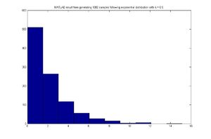
MATLAB result

Discrete Case-Sept 22, 2011

This same technique can be applied to the discrete case. Generate a discrete random variable [math]\displaystyle{ \,x }[/math] that has probability mass function [math]\displaystyle{ \,P(X=x_i)=P_i }[/math] where [math]\displaystyle{ \,x_0\lt x_1\lt x_2... }[/math] and [math]\displaystyle{ \,\sum_i P_i=1 }[/math]

• Step 1. Draw [math]\displaystyle{ u \sim~ \mathrm{Unif}[0, 1] }[/math]
• Step 2. [math]\displaystyle{ \,x=x_i }[/math] if [math]\displaystyle{ \,F(x_{i-1})\lt u \leq F(x_i) }[/math]

Example

Let x be a discrete random variable with the following probability mass function:

[math]\displaystyle{ \begin{align} P(X=0) = 0.3 \\ P(X=1) = 0.2 \\ P(X=2) = 0.5 \end{align} }[/math]

Given the pmf, we now need to find the cdf.

We have:

[math]\displaystyle{ F(x) = \begin{cases} 0 & x \lt 0 \\ 0.3 & 0 \leq x \lt 1 \\ 0.5 & 1 \leq x \lt 2 \\ 1 & 2 \leq x \end{cases} }[/math]

We can apply the inverse transform method to obtain our random numbers from this distribution.

Pseudo Code for generating the random numbers:

Draw U ~ Unif[0,1] 
     if U <= 0.3 
        x = 0 
     else if  
        0.3 < U <= 0.5 
        x = 1 
     else 
        0.5 < U <= 1 
        x = 2

MATLAB code for generating 1000 random numbers in the discrete case:

for ii = 1:1000
    u = rand;
    
    if u <= 0.3
       x(ii) = 0;
       else if u <= 0.5
           x(ii) = 1;
           else
             x(ii) = 2;
    end
end

Pseudo code for the Discrete Case:

1. Draw U ~ Unif [0,1]

2. If [math]\displaystyle{ U \leq P_0 }[/math], deliver [math]\displaystyle{ X = x_0 }[/math]

3. Else if [math]\displaystyle{ U \leq P_0 + P_1 }[/math], deliver [math]\displaystyle{ X = x_1 }[/math]

4. Else If [math]\displaystyle{ U \leq P_0 +....+ P_k }[/math], deliver [math]\displaystyle{ X = x_k }[/math]

Limitations

Although this method is useful, it isn't practical in many cases since we can't always obtain [math]\displaystyle{ F }[/math] or [math]\displaystyle{ F^{-1} }[/math] as some functions are not integrable or invertible, and sometimes even [math]\displaystyle{ f(x) }[/math] itself cannot be obtained in closed form. Let's look at some examples:

• Continuous case

If we want to use this method to draw the pdf of normal distribution, we may find ourselves get stuck in finding its cdf. The simplest case of normal distribution is [math]\displaystyle{ f(x)=\frac{1}{\sqrt{2\pi}}e^{-\frac{x^2}{2}} }[/math], whose cdf is [math]\displaystyle{ F(x)=\frac{1}{\sqrt{2\pi}}\int_{-\infty}^{x}{e^{-\frac{u^2}{2}}}du }[/math]. This integral cannot be expressed in terms of elementary functions. So evaluating it and then finding the inverse is a very difficult task.

• Discrete case

It is easy for us to simulate when there are only a few values taken by the particular random variable, like the case above. And it is easy to simulate the binomial distribution [math]\displaystyle{ X \sim~ \mathrm{B}(n,p) }[/math] when the parameter n is not too large. But when n takes on values that are very large, say 50, it is hard to do so.

Acceptance/Rejection Method

The aforementioned difficulties of the inverse transform method motivates a sampling method that does not require analytically calculating cdf's and their inverses, which is the acceptance/rejection sampling method. Here, [math]\displaystyle{ f(x) }[/math] is approximated by another function, say [math]\displaystyle{ g(x) }[/math], with the idea being that [math]\displaystyle{ g(x) }[/math] is a "nicer" function to work with than [math]\displaystyle{ f(x) }[/math].

Suppose we assume the following:

1. There exists another distribution [math]\displaystyle{ g(x) }[/math] that is easier to work with and that you know how to sample from, and

2. There exists a constant c such that [math]\displaystyle{ f(x) \leq c \cdot g(x) }[/math] for all x

Under these assumptions, we can sample from [math]\displaystyle{ f(x) }[/math] by sampling from [math]\displaystyle{ g(x) }[/math]

General Idea

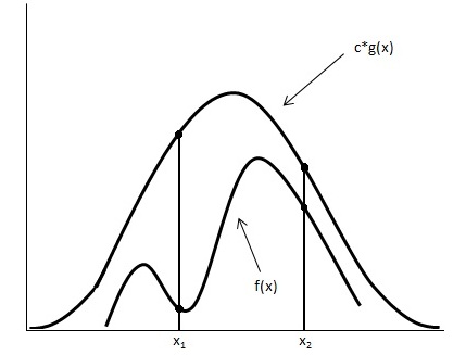
Looking at the image below we have graphed [math]\displaystyle{ c \cdot g(x) }[/math] and [math]\displaystyle{ f(x) }[/math].

Using the acceptance/rejection method we will accept some of the points from [math]\displaystyle{ g(x) }[/math] and reject some of the points from [math]\displaystyle{ g(x) }[/math]. The points that will be accepted from [math]\displaystyle{ g(x) }[/math] will have a distribution similar to [math]\displaystyle{ f(x) }[/math]. We can see from the image that the values around [math]\displaystyle{ x_1 }[/math] will be sampled more often under [math]\displaystyle{ c \cdot g(x) }[/math] than under [math]\displaystyle{ f(x) }[/math], so we will have to reject more samples taken at x₁. Around [math]\displaystyle{ x_2 }[/math] the number of samples that are drawn and the number of samples we need are much closer, so we accept more samples that we get at [math]\displaystyle{ x_2 }[/math]

Procedure

1. Draw y ~ g

2. Draw U ~ Unif [0,1]

3. If [math]\displaystyle{ U \leq \frac{f(y)}{c \cdot g(y)} }[/math] then x=y; else return to 1

Proof

Mathematically, we need to show that the sample points given that they are accepted have a distribution of f(x).

[math]\displaystyle{ \begin{align} P(y|accepted) &= \frac{P(y, accepted)}{P(accepted)} \\ &= \frac{P(accepted|y) P(y)}{P(accepted)}\end{align} }[/math] (Bayes' Rule)

[math]\displaystyle{ P(y) = g(y) }[/math]

[math]\displaystyle{ P(accepted|y) =P(u\leq \frac{f(y)}{c \cdot g(y)}) =\frac{f(y)}{c \cdot g(y)} }[/math],where u ~ Unif [0,1]

[math]\displaystyle{ P(accepted) = \sum P(accepeted|y)\cdot P(y)=\int^{}_y \frac{f(y)}{c \cdot g(y)}g(y) dy=\int^{}_y \frac{f(y)}{c} dy=\frac{1}{c} \cdot\int^{}_y f(y) dy=\frac{1}{c} }[/math]

So,

[math]\displaystyle{ P(y|accepted) = \frac{ \frac {f(y)}{c \cdot g(y)} \cdot g(y)}{\frac{1}{c}} =f(y) }[/math]

Continuous Case

Example

Sample from Beta(2,1)

In general:

Beta([math]\displaystyle{ \alpha, \beta) = \frac{\Gamma (\alpha + \beta)}{\Gamma(\alpha)\Gamma(\beta)} }[/math] [math]\displaystyle{ x^{\alpha-1} }[/math] [math]\displaystyle{ (1-x)^{\beta-1} }[/math], [math]\displaystyle{ 0\lt x\lt 1 }[/math]

Note: [math]\displaystyle{ \Gamma(n) = (n-1)! }[/math] if n is a positive integer

[math]\displaystyle{ \begin{align} f(x) &= Beta(2,1) \\ &= \frac{\Gamma(3)}{\Gamma(2)\Gamma(1)} x^1(1-x)^0 \\ &= \frac{2!}{1! 0!}\cdot (1) x \\ &= 2x \end{align} }[/math]

We want to choose [math]\displaystyle{ g(x) }[/math] that is easy to sample from. So we choose [math]\displaystyle{ g(x) }[/math] to be uniform distribution.

We now want a constant c such that [math]\displaystyle{ f(x) \leq c \cdot g(x) }[/math] for all x from (0,1)

So,

[math]\displaystyle{ c \geq \frac{f(x)}{g(x)} }[/math], for all x from (0,1)

[math]\displaystyle{ \begin{align}c &\geq max (\frac {f(x)}{g(x)}, 0\lt x\lt 1) \\ &= max (\frac {2x}{1},0\lt x\lt 1) \\ &= 2 \end{align} }[/math]

Now that we have c =2,

1. Draw y ~ g(x) => Draw y ~ Unif [0,1]

2. Draw u ~ Unif [0,1]

3. if [math]\displaystyle{ u \leq \frac{2y}{2 \cdot 1} }[/math] then x=y; else return to 1

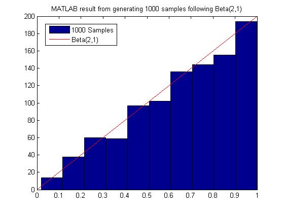
MATLAB code for generating 1000 samples following Beta(2,1):

close all
clear all
ii=1;
while ii < 1000
    y = rand;
    u = rand;
    
    if u <= y
        x(ii)=y;
        ii=ii+1;
    end
end
hist(x)

MATLAB result

Discrete Example

Generate random variables according to the p.m.f:

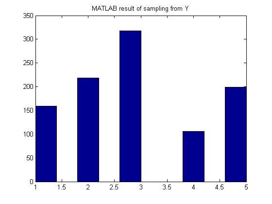
[math]\displaystyle{ \begin{align} P(Y=1) = 0.15 \\ P(Y=2) = 0.22 \\ P(Y=3) = 0.33 \\ P(Y=4) = 0.10 \\ P(Y=5) = 0.20 \end{align} }[/math]

find a g(y) discrete uniform distribution from 1 to 5

[math]\displaystyle{ c \geq \frac{P(y)}{g(y)} }[/math]
[math]\displaystyle{ c = \max \left(\frac{P(y)}{g(y)} \right) }[/math]
[math]\displaystyle{ c = \max \left(\frac{0.33}{0.2} \right) = 1.65 }[/math] Since P(Y=3) is the max of P(Y) and g(y) = 0.2 for all y.

1. Generate Y according to the discrete uniform between 1 - 5

2. U ~ unif[0,1]

3. If [math]\displaystyle{ U \leq \frac{P(y)}{1.65 \times 0.2} \leq \frac{P(y)}{0.33} }[/math], then x = y; else return to 1.

In MATLAB, the code would be:

   py = [0.15 0.22 0.33 0.1 0.2];
   ii =1;
   while ii <= 1000
       y = unidrnd(5);
       u = rand;
       if u <= py(y)/0.33
           x(ii) = y;
           ii = ii+1;
       end
   end
   hist(x);

MATLAB result

Limitations

Most of the time we have to sample many more points from g(x) before we can obtain an acceptable amount of samples from f(x), hence this method may not be computationally efficient. It depends on our choice of g(x). For example, in the example above to sample from Beta(2,1), we need roughly 2000 samples from g(X) to get 1000 acceptable samples of f(x).

Sampling From Gamma and Normal Distribution - Sept 27, 2011

Sampling From Gamma

Gamma Distribution

The Gamma function is written as [math]\displaystyle{ X \sim~ Gamma (t, \lambda) }[/math]

[math]\displaystyle{ F(x) = \int_{0}^{\lambda x} \frac{e^{-y}y^{t-1}}{(t-1)!} dy }[/math]

If you have t samples of the exponential distribution,

[math]\displaystyle{ \begin{align} X_1 \sim~ Exp(\lambda)\\ \vdots \\ X_t \sim~ Exp(\lambda) \end{align} }[/math]

The sum of these t samples has a gamma distribution,

[math]\displaystyle{ X_1+X_2+ ... + X_t \sim~ Gamma (t, \lambda) }[/math]

[math]\displaystyle{ \sum_{i=1}^{t} X_i \sim~ Gamma (t, \lambda) }[/math] where [math]\displaystyle{ X_i \sim~Exp(\lambda) }[/math]

method

We can sample the exponential distribution using the inverse transform method from previous class,

[math]\displaystyle{ \,f(x)={\lambda}e^{-{\lambda}x} }[/math]

[math]\displaystyle{ \,F^{-1}(u)=\frac{-ln(1-u)}{\lambda} }[/math]

[math]\displaystyle{ \,F^{-1}(u)=\frac{-ln(u)}{\lambda} }[/math]

1 - u is the same as x since [math]\displaystyle{ U \sim~ unif [0,1] }[/math]

[math]\displaystyle{ \begin{align} \frac{-ln(u_1)}{\lambda} - \frac{ln(u_2)}{\lambda} - ... - \frac{ln(u_t)}{\lambda} = x_1\\ \vdots \\ \frac{-ln(u_1)}{\lambda} - \frac{ln(u_2)}{\lambda} - ... - \frac{ln(u_t)}{\lambda} = x_t \end{align}  : }[/math]

[math]\displaystyle{ \frac {-\sum_{i=1}^{t} ln(u_i)}{\lambda} = x }[/math]

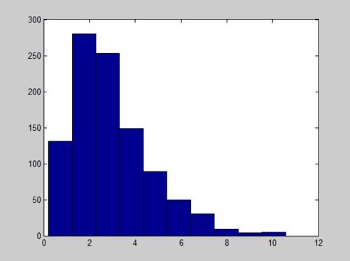
MATLAB code for a Gamma(1,3) is

x = sum(-log(rand(1000,3)),2); 
hist(x)

And the Histogram of X follows a Gamma distribution with long tail:

R code for a Gamma(1,3) is

a<-apply(-log(matrix(runif(3000),nrow=1000)),1,sum);
hist(a);

And the histogram is

File:hist gamma.png

Here is another histogram of Gamma coding with R

a<-apply(-log(matrix(runif(3000),nrow=1000)),1,sum);
hist(a,freq=F);
lines(density(a),col="blue");
rug(jitter(a));

File:hist gamma 2.png

Sampling From Normal Distribution

Box-Muller Transform - Sept 29, 2011

Procedure

1. Generate [math]\displaystyle{ u_1 }[/math] and [math]\displaystyle{ u_1 }[/math], two values sampled from a uniform distribution between 0 and 1.

2.

   Set [math]\displaystyle{ R^2 = -2log(u_1) }[/math] so that [math]\displaystyle{ R^2 }[/math] is exponential with mean 1/2

   Set [math]\displaystyle{ \theta = 2*\pi*u_2 }[/math] so that [math]\displaystyle{ \theta }[/math] ~ Unif[0, 2[math]\displaystyle{ \pi }[/math]]

3.

   Set [math]\displaystyle{ X = R cos(\theta) }[/math]

   Set [math]\displaystyle{ Y = R sin(\theta) }[/math]

Justification

Suppose we have X ~ N(0, 1) and Y ~ N(0, 1). The relative probability density function of these two random variables using Cartesian coordinates is:

[math]\displaystyle{ f(X, Y) = f(X) f(Y) = \frac{1}{\sqrt{2\pi}}e^{-x^2/2} \frac{1}{\sqrt{2\pi}}e^{-y^2/2} = \frac{1}{2\pi}e^{-(x^2+y^2)/2} }[/math]

In polar coordinates [math]\displaystyle{ R^2 = x^2 + y^2 }[/math], so the relative probability density function of these two random variables using polar coordinates is:

[math]\displaystyle{ f(R, \theta) = \frac{1}{2\pi}e^{-R^2/2} }[/math]

If we have [math]\displaystyle{ R^2 }[/math] ~ exp(1/2) and [math]\displaystyle{ \theta }[/math] ~ unif[0, 2[math]\displaystyle{ \pi }[/math]] we get an equivalent relative probability density function:

[math]\displaystyle{ f(R, \theta) = f(R) f(\theta) = \frac{1}{2}e^{-R^2/2} * \frac{1}{2\pi} = \frac{1}{4\pi}e^{-R^2/2} }[/math]

Therefore we can generate a point in polar coordinates using the uniform and exponential distributions, then convert the point to Cartesian coordinates and the resulting X and Y values will be equivalent to samples generated from N(0, 1).

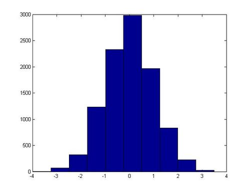
MATLAB code In MatLab this algorithm can be implemented with the following code, which generates 20,000 samples from N(0, 1):

x = zeros(10000, 1);
y = zeros(10000, 1);
for ii = 1:10000
    u1 = rand;
    u2 = rand;
    R2 = -2 * log(u1);
    theta = 2 * pi * u2;
    x(ii) = sqrt(R2) * cos(theta);
    y(ii) = sqrt(R2) * sin(theta);
end
hist(x)

In one execution of this script, the following histogram for x was generated:

Non-Standard Normal Distributions

Example: with Co-Variance=0

If X ~ Norm(0, 1) then (a + bX) has a normal distribution with a mean of a and a standard deviation of b (which is equivalent to a variance of [math]\displaystyle{ b^2 }[/math]). Using this information with the Box-Muller transform, we can generate values sampled from some random variable Y ~ Norm(a, [math]\displaystyle{ b^2 }[/math]) for arbitrary values of a and b.

1. Generate a sample u from Norm(0, 1) using the Box-Muller transform.

2. Set v = a + bu.

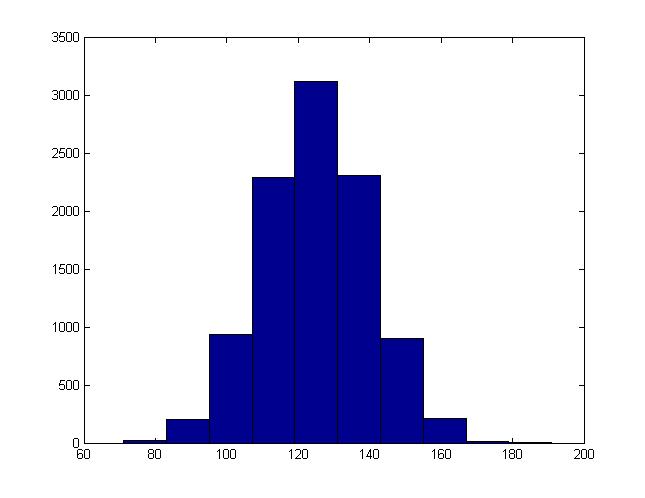
The values for v generated in this way will be equivalent to samples from a Norm(a, [math]\displaystyle{ b^2 }[/math]) distribution. We can modify the MatLab code used in the last section to demonstrate this. We just need to add one line before we generate the histogram:

x = b + a * x;

For instance, this is the histogram generated when b = 15, a = 125:

500

Example2: with Co-Variance>0

Where:

 -  [math]\displaystyle{ \mathbf{u} }[/math] is an n by 1 vector
 -  [math]\displaystyle{ \Sigma }[/math] is an n by n matrix
 -  [math]\displaystyle{ 1 \leq i, j \leq n }[/math]

[math]\displaystyle{ \mathbf{z} = N(\mathbf{u}, \Sigma) }[/math] defines the n by 1 vector [math]\displaystyle{ \mathbf{z} }[/math] such that:

 -  ui is the average of zi
 -  [math]\displaystyle{ \Sigma }[/math]ii is the variance of zi
 -  [math]\displaystyle{ \Sigma }[/math]ij is the co-variance of zi and zj

We can compute [math]\displaystyle{ \mathbf{z} }[/math] in the following way:

1. Generate an n by 1 vector [math]\displaystyle{ \mathbf{x} = \begin{bmatrix}x_{1} & x_{2} & ... & x_{n}\end{bmatrix} }[/math] where [math]\displaystyle{ x_{1} }[/math] ~ Norm(0, 1) using the Box-Muller transform.

2. Calculate [math]\displaystyle{ \Sigma^\frac{1}{2} }[/math] using singular value decomposition.

3. Set [math]\displaystyle{ \mathbf{z} = \Sigma^\frac{1}{2} \mathbf{x} + \mathbf{u} }[/math].

x = zeros(10000, 1);
y = zeros(10000, 1);
for ii = 1:10000
    u1 = rand;
    u2 = rand;
    R2 = -2 * log(u1);
    theta = 2 * pi * u2;
    x(ii) = sqrt(R2) * cos(theta);
    y(ii) = sqrt(R2) * sin(theta);
end

E = [1, 0.9; 0.9, 1];
[u s v] = svd(E);
root_E = u * (s ^ (1 / 2));

z = (root_E * [x y]')';
z(:,1) = z(:,1) + 5;
z(:,1) = z(:,1) + -8;

scatter(z(:,1), z(:,2))

This code generated the following scatter plot: // In progress

File:scatter covar.jpg

R code for a multivariate normal distribution

n=10000;
r2<--2*log(runif(n));
theta<-2*pi*(runif(n));
x<-sqrt(r2)*cos(theta);
y<-sqrt(r2)*sin(theta);
a<-matrix(c(x,y),nrow=n,byrow=F);
e<-matrix(c(1,.9,09,1),nrow=2,byrow=T);
svde<-svd(e);
root_e<-svde$u %*% diag(svde$d)^1/2;
z<-t(root_e %*%t(a));
z[,1]=z[,1]+5;
z[,2]=z[,2]+ -8;
par(pch=19);
plot(z,col=rgb(1,0,0,alpha=0.06))

File:m normal.png

Sampling From Binomial Distributions

In order to generate a sample x from X ~ Bin(n, p), we can follow the following procedure:

1. Generate n uniform random numbers sampled from Unif[0, 1]: [math]\displaystyle{ u_1, u_2, ..., u_n }[/math].

2. Set x to be the total number of cases where [math]\displaystyle{ u_i \lt = p }[/math] for all [math]\displaystyle{ 1 \lt = i \lt = n }[/math].

In MatLab this can be coded with a single line. The following generates a sample from X ~ Bin(n, p):

>> sum(rand(n, 1) <= p, 1)

For instance, sum(rand(10000, 1) <= 0.2, 1) samples from X ~ Bin(10000, 0.2).