Research Papers Classification System

Please Do NOT Edit This Summary

This is just a draft!

Presented by

Jill Wang, Junyi (Jay) Yang, Yu Min (Chris) Wu, Chun Kit (Calvin) Li

Introduction

This paper introduces a paper classification system that utilizes the Term frequency-inverse document frequency (TF-IDF), Latent Dirichlet Allocation (LDA), and K-means clustering. The most important technology the system used to process big data is the Hadoop Distributed File Systems (HDFS). The system can handle quantitatively complex research paper classification problems efficiently and accurately.

General Framework

The paper classification system classifies research papers based on the abstracts given that the core of most papers is presented in the abstracts.

1. Paper Crawling

   Collects abstracts from research papers published during a given period

2. Preprocessing
   1. Removes stop words in the papers crawled, in which only nouns are extracted from the papers
   2. generates a keyword dictionary, keeping only the top-N keywords with the highest frequencies

3. Topic Modelling

   Use the LDA to group the keywords into topics

4. Paper Length Calculation

   Calculates the total number of occurrences of words to prevent an unbalanced TF values caused by the various length of abstracts using the map-reduce algorithm

5. Word Frequency Calculation

   Calculates the Term Frequency (TF) values which represent the frequency of keywords in a research paper

6. Document Frequency Calculation

   Calculates the Document Frequency (DF) values which represents the frequency of keywords in a collection of research papers. The higher the DF value, the lower the importance of a keyword.

7. TF-IDF calculation

   Calculates the inverse of the DF which represents the importance of a keyword.

8. Paper Classification

   Classify papers by topics using the K-means clustering algorithm.

Technologies

The HDFS with a Hadoop cluster composed of one master node, one sub node, and four data nodes is what is used to process the massive paper data. Hadoop-2.6.5 version in Java is what is used to perform the TF-IDF calculation. Spark MLlib is what is used to perform the LDA. The Scikit-learn library is what is used to perform the K-means clustering.

HDFS

Hadoop Distributed File Systems was used to process big data in this system. What Hadoop does is to break a big collection of data into different partitions and pass each partition to one individual processor. Each processor will only have information about the partition of data it received.

In this summary, we are going to focus on introducing the main algorithms of what this system uses, namely LDA, TF-IDF, and K-Means.

Data Preprocessing

Crawling of Abstract Data

Under the assumption that audiences tend to first read the abstract of papers to gain an understanding of the papers. As a result, the abstract of any paper may include “core words” that can be used to effectively classify papers’ subjects.

An abstract is crawled to have its stop words removed. Stop words are words that are usually ignored by search engines, such as “the”, “a”, and etc. Afterwards, nouns are extracted, as a more condensed representation for efficient analysis.

Managing Paper Data

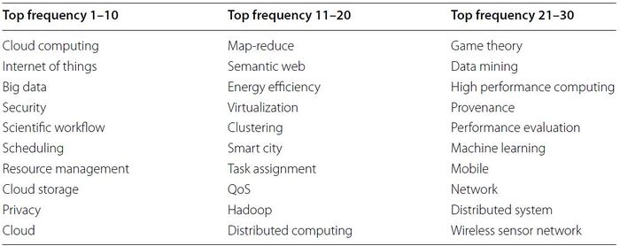
To construct an effective keyword dictionary using abstract data and keywords data in all of the crawled papers, the authors categorized keywords with similar meanings using a single representative keyword. The approach is called stemming, which is common in cleaning data. 1394 keyword categories are extracted, which is still too much to compute. Hence, only the top 30 keyword categories are used.

Topic Modeling Using LDA

Latent Dirichlet allocation (LDA) is a generative probabilistic model that views documents as random mixtures over latent topics. Each topic is a distribution over words, and the goal is to extract these topics from documents.

LDA estimates the topic-word distribution [math]\displaystyle{ P\left(t | z\right) }[/math] and the document-topic distribution [math]\displaystyle{ P\left(z | d\right) }[/math] using Dirichlet priors for the distributions with a fixed number of topics. For each document, obtain a feature vector:

\[F = \left( P\left(z_1 | d\right), P\left(z_2 | d\right), \cdots, P\left(z_k | d\right) \right)\]

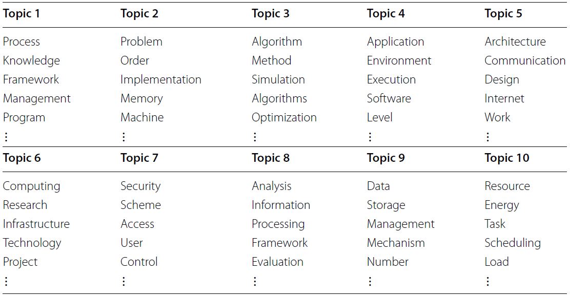
In the paper, authors extract topics from preprocessed paper to generate three kinds of topic sets, each with 10, 20, and 30 topics respectively. The following is a table of the 10 topic sets of highest frequency keywords.

LDA Intuition

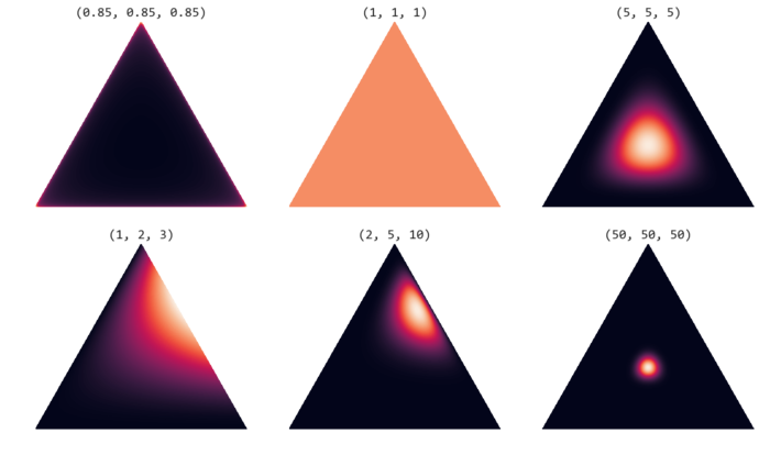
LDA uses the Dirichlet priors of the Dirichlet distribution. The following picture illustrates 2-simplex Dirichlet distributions with different alpha values, one for each corner of the triangles.

Simplex is a generalization of the notion of a triangle. In Dirichlet distribution, each parameter will be represented by a corner in simplex, so adding additional parameters implies increasing the dimensions of simplex. As illustrated, when alphas are smaller than 1 the distribution is dense at the corners. When the alphas are greater than 1 the distribution is dense at the centers.

The following illustration shows an example LDA with 3 topics, 4 words and 7 documents.

In the left diagram, there are three topics, hence it is a 2-simplex. In the right diagram there are four words, hence it is a 3-simplex. LDA essentially adjusts parameters in Dirichlet distributions and multinomial distributions (represented by the points), such that, in the left diagram, all the yellow points representing documents and, in the right diagram, all the points representing topics, are as close to a corner as possible. In other words, LDA finds topics for documents and also finds words for topics. At the end topic-word distribution [math]\displaystyle{ P\left(t | z\right) }[/math] and the document-topic distribution [math]\displaystyle{ P\left(z | d\right) }[/math] are produced.

Term Frequency Inverse Document Frequency (TF-IDF) Calculation

TF-IDF is widely used to evaluate the importance of a set of words in the fields of information retrieval and text mining. It is a combination of term frequency (TF) and inverse document frequency (IDF). The idea behind this combination is It evaluates the importance of a word within a document, and It evaluates the importance of the word among the collection of all documents

The TF-IDF formula has the following form:

\[TF-IDF_{i,j} = TF_{i,j} \times IDF_{i}\]

where i stands for the [math]\displaystyle{ i^{th} }[/math] word and j stands for the [math]\displaystyle{ j^{th} }[/math] document.

Term Frequency (TF)

TF evaluates the percentage of a given word in a document. Thus, TF value indicates the importance of a word. The TF has a positive relation with the importance.

In this paper, we only calculate TF for words in the keyword dictionary obtained. For a given keyword i, [math]\displaystyle{ TF_{i,j} }[/math] is the number of times word i appears in document j divided by the total number of words in document j.

The formula for TF has the following form:

\[TF_{i,j} = \frac{n_{i,j} }{\sum_k n_{k,j} }\]

where i stands for the [math]\displaystyle{ i^{th} }[/math] word, j stands for the [math]\displaystyle{ j^{th} }[/math] document, and [math]\displaystyle{ n_{i,j} }[/math] stands for the number of times words i appear in document j.

Note that the denominator is the total number of words remaining in document j after crawling.

Document Frequency (DF)

DF evaluates the percentage of documents that contain a given word over the entire collection of documents. Thus, the higher DF value is, the less important the word is. Since DF and the importance of the word have an inverse relation, we use IDF instead of DF.

[math]\displaystyle{ DF_{i} }[/math] is the number of documents in the collection with word i divided by the total number of documents in the collection. The formula for DF has the following form:

\[DF_{i} = \frac{|d_k \in D: n_{i,k} > 0|}{|D|}\]

where [math]\displaystyle{ n_{i,k} }[/math] is the number of times word i appears in document k, |D| is the total number of documents in the collection.

Inverse Document Frequency (IDF)

In this paper, IDF is calculated in a log scale. Since we will receive a large number of documents, i.e, we will have a large |D|

The formula for IDF has the following form:

\[IDF_{i} = log\left(\frac{|D|}{|\{d_k \in D: n_{i,k} > 0\}|}\right)\]

As mentioned before, we will use HDFS. The actual formula applied is:

\[IDF_{i} = log\left(\frac{|D|+1}{|\{d_k \in D: n_{i,k} > 0\}|+1}\right)\]

Paper Classification Using K-means Clustering

The K-means clustering is an unsupervised classification algorithm that groups similar data into the same class. It is an efficient and simple method that can work with different types of data attributes and is able to handle noise and outliers.

Given a set of [math]\displaystyle{ d }[/math] by [math]\displaystyle{ n }[/math] dataset [math]\displaystyle{ \mathbf{X} = \left[ \mathbf{x}_1 \cdots \mathbf{x}_n \right] }[/math], the algorithm will assign each [math]\displaystyle{ \mathbf{x}_j }[/math] into [math]\displaystyle{ k }[/math] different clusters based on the characteristics of [math]\displaystyle{ \mathbf{x}_j }[/math] itself.

Moreover, when assigning data into a cluster, the algorithm will also try to minimise the distances between the data and the centre of the cluster which the data belongs to. That is, k-means clustering will minimise the sum of square error:

\begin{align*} min \sum_{i=1}^{k} \sum_{j \in C_i} ||x_j - \mu_i||^2 \end{align*}

where

• [math]\displaystyle{ k }[/math]: the number of clusters
• [math]\displaystyle{ C_i }[/math]: the [math]\displaystyle{ i^th }[/math] cluster
• [math]\displaystyle{ x_j }[/math]: the [math]\displaystyle{ j^th }[/math] data in the [math]\displaystyle{ C_i }[/math]
• [math]\displaystyle{ mu_i }[/math]: the centroid of [math]\displaystyle{ C_i }[/math]
• [math]\displaystyle{ ||x_j - \mu_i||^2 }[/math]: the Euclidean distance between [math]\displaystyle{ x_j }[/math] and [math]\displaystyle{ \mu_i }[/math]

Since the goal for this paper is to classify research papers and group papers with similar topics based on keywords, the paper uses the K-means clustering algorithm. The algorithm first computes the cluster centroid for each group of papers with a specific topic. Then, it will assign a paper into a cluster based on the Euclidean distance between the cluster centroid and the paper’s TF-IDF value.

However, different values of [math]\displaystyle{ k }[/math] (the number of clusters) will return different clustering results. Therefore, it is important to define the number of clusters before clustering. For example, in this paper, the authors choose to use the Elbow scheme to determine the value of [math]\displaystyle{ k }[/math]. Also, to measure the performance of clustering, the authors decide to use the Silhouette scheme. The results of clustering are validated if the Silhouette scheme returns a value greater than [math]\displaystyle{ 0.5 }[/math].

System Testing Results

In this paper, the dataset has 3264 research papers from the Future Generation Computer System (FGCS) journal between 1984 and 2017. For constructing keyword dictionaries for each paper, the authors have introduced three methods as shown below:

Then, the authors use the Elbow scheme to define the number of clusters for each method with different numbers of keywords before running the K-means clustering algorithm. The results are shown below:

According to table 4, there is a positive correlation between the number of keywords and the number of clusters. In addition, method 3 combines the advantages for both method 1 and method 2; thus, method 3 requires the least clusters in total. On the other hand, the wrong keywords might be presented in papers; hence, it might not be possible to group papers with similar subjects correctly by using method 1 and so method 1 needs the most number of clusters in total.

Next, the Silhouette scheme had been used for measuring the performance for clustering. The average of the Silhouette values for each method with different numbers of keywords are shown below:

Since the clustering is validated if the Silhouette’s value is greater than 0.5, for methods with 10 and 30 keywords, the K-means clustering algorithm produces good results.

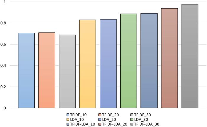
To evaluate the accuracy of the classification system in this paper, the authors use the F-Score. The authors execute 5 times of experiment and use 500 randomly selected research papers for each trial. The following histogram shows the average value of F-Score for the three methods and different numbers of keywords:

Note that “TFIDF” means method 1, “LDA” means method 2, and “TFIDF-LDA” means method 3. The number 10, 20, and 30 after each method is the number of keywords the method has used. According to the histogram above, method 3 has the highest F-Score values than the other two methods with different numbers of keywords. Therefore, the classification system is most accurate when using method 3 as it combines the advantages for both method 1 and method 2.

Conclusion

This paper introduces a classification system that classifies papers into different topics by using TF-IDF and LDA scheme with K-means clustering algorithm. This system allows users to search the papers they want quickly and with the most productivity.

Furthermore, this classification system might be also used in different types of texts (e.g. documents, tweets, etc.) instead of only classifying research papers.

Critique

In this paper, DF values are calculated within each partition. The authors introduced a dummy document to avoid running into dividing by zero problems. Another method to deal with this is to have all partition to communicate with their DF value. Then pass the merged DF value to all partitions to do the final IDF and TF-IDF value.

References

Kim, SW., Gil, JM. (2019). Research paper classification systems based on TF-IDF and LDA schemes. Human-centric Computing and Information Sciences, 9, 30 (2019). https://doi.org/10.1186/s13673-019-0192-7