THE LOGICAL EXPRESSIVENESS OF GRAPH NEURAL NETWORKS

Presented By

Abhinav Jain

Background

Graph neural networks (GNNs) (Merkwirth & Lengauer, 2005; Scarselli et al., 2009) are a class of neural network architectures that have recently become popular for a wide range of applications dealing with structured data, e.g., molecule classification, knowledge graph completion, and Web page ranking (Battaglia et al., 2018; Gilmer et al., 2017; Kipf & Welling, 2017; Schlichtkrull et al., 2018). The main idea behind GNNs is that the connections between neurons are not arbitrary but reflect the structure of the input data. This approach is motivated by convolutional and recurrent neural networks and generalizes both of them (Battaglia et al., 2018). Despite the fact that GNNs have recently been proven very efficient in many applications, their theoretical properties are not yet well-understood.

The ability of graph neural networks (GNNs) for distinguishing nodes in graphs has been recently characterized in terms of the Weisfeiler-Lehman (WL) test for checking graph isomorphism. The WL test works by constructing labeling of the nodes of the graph, in an incremental fashion, and then decides whether two graphs are isomorphic by comparing the labeling of each graph. This characterization, however, does not settle the issue of which Boolean node classifiers (i.e., functions classifying nodes in graphs as true or false) can be expressed by GNNs. To state the connection between GNNs and this test, consider the simple GNN architecture that updates the feature vector of each graph node by combining it with the aggregation of the feature vectors of its neighbors. We call such GNNs aggregate-combine GNNs, or AC-GNNs. Moreover, there are AC-GNNs that can reproduce the WL labeling. This does not imply, however, that AC-GNNs can capture every node classifier—that is, a function assigning true or false to every node—that is refined by the WL test. The author's work aims to answer the question of what are the node classifiers that can be captured by GNN architectures such as AC-GNNs.

Image: 500 pixels

Figure 2: Certified Defense Illustration

Introduction

They tackle this problem by focusing on Boolean classifiers expressible as formulas in the logic FOC2, a well-studied fragment of first-order logic. FOC2 is tightly related to the WL test, and hence to GNNs. They start by studying a popular class of GNNs, which they call AC-GNNs, in which the features of each node in the graph are updated, in successive layers, only in terms of the features of its neighbors.

Given the connection between AC-GNNs and WL on the one hand, and that between WL and FOC2 on the other hand, one may be tempted to think that the expressivity of AC-GNNs coincides with that of FOC2. However, the reality is not as simple, and there are many FOC2 node classifiers (e.g., the trivial one above) that cannot be expressed by AC-GNNs. This leaves us with the following natural questions. First, what is the largest fragment of FOC2 classifiers that can be captured by AC-GNNs? Second, is there an extension of AC-GNNs that allows expressing all FOC2 classifiers? In this paper, they provide answers to these two questions.

The following are the main contributions:

1. They characterize exactly the fragment of FOC2 formulas that can be expressed as ACGNNs. This fragment corresponds to graded modal logic (de Rijke, 2000), or, equivalently, to the description logic ALCQ, which has received considerable attention in the knowledge representation community (Baader et al., 2003; Baader & Lutz, 2007).

2. Next, they extend the AC-GNN architecture in a very simple way by allowing global readouts, wherein each layer they also compute a feature vector for the whole graph and combine it with local aggregations; they call these aggregate-combine-readout GNNs (ACR-GNNs). These networks are a special case of the ones proposed by Battaglia et al. (2018) for relational reasoning over graph representations. In this setting, they prove that each FOC2 formula can be captured by an ACR-GNN.

They experimentally validate our findings showing that the theoretical expressiveness of ACR-GNNs, as well as the differences between AC-GNNs and ACR-GNNs, can be observed when they learn from examples. In particular, they show that on synthetic graph data conforming to FOC2 formulas, ACGNNs struggle to fit the training data while ACR-GNNs can generalize even to graphs of sizes not seen during training.

Approach

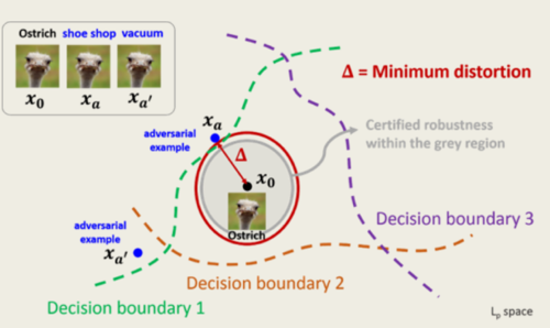
The approach used by the authors in this paper is 'Shadow Attack', which is a generalization of the well known Projected Gradient Descent (PGD) attack. PGD, a universal first-order adversary [4], is the only method to greatly improve NN model robustness among all the defenses appearing in ICLR2018 and CVPR2018 [5]. The fundamental idea of the PGD attack is the same where a bunch of adversarial images is created in order to fool the network to make a wrong prediction. PGD attack solves the following optimization problem where [math]\displaystyle{ L }[/math] is the classification loss and the constraint corresponds to the minimal change done to the input image. For a recent review on adversarial attacks and more information on PGD attacks, see [1].

\begin{align} max_{\delta }L\left ( \theta, x + \delta \right ) \tag{1} \label{eq:op} \end{align}

\begin{align} s.t. \left \|\delta \right \|_{p} \leq \epsilon \end{align}

Shadow attack on the other hand targets the certificate of the defenses by creating a new 'spoofed' certificate outside the certificate region of the input image. Shadow attack solves the following optimization problem where [math]\displaystyle{ C }[/math], [math]\displaystyle{ TV }[/math], and [math]\displaystyle{ Dissim }[/math] are the regularizers.

\begin{align} max_{\delta} L\left (\theta ,x+\delta \right ) - \lambda_{c}C\left (\delta \right )-\lambda_{tv}TV\left ( \delta \right )-\lambda_{s}Dissim\left ( \delta \right ) \tag{2} \label{eq:op1} \end{align}

In equation \eqref{eq:op1}, [math]\displaystyle{ C }[/math] in the above equation corresponds to the color regularizer which makes sure that minimal changes are made to the color of the input image. [math]\displaystyle{ TV }[/math] corresponds to the Total Variation or smoothness parameter which makes sure that the smoothness of the newly created image is maintained. [math]\displaystyle{ Dissim }[/math] corresponds to the similarity parameter which makes sure that all the color channels (RGB) are changed equally.

The perturbations created in the original images are -

1. small

2. smooth

3. without dramatic color changes

There are two ways to ensure that this dissimilarity will not happen or will be very low and the authors have shown that both of these methods are effective.

• 1-channel attack: This strictly enforces [math]\displaystyle{ \delta_{R,i} \approx \delta_{G,i} \approx \delta_{B,i} \forall i }[/math] i.e. for each pixel, the perturbations of all channels are equal and there will be [math]\displaystyle{ \delta_{ W \times H} }[/math], where the size of the image is [math]\displaystyle{ 3 \times W \times H }[/math] as the preturbation. In this case, [math]\displaystyle{ Dissim(\delta)=0 }[/math].

• 3-channel attack: In this kind of attack, the perturbations in different channels of a pixel are not equal and it uses [math]\displaystyle{ \delta_{3 \times W \times H} }[/math] with the [math]\displaystyle{ Dissim(\delta) = || \delta_{R}- \delta_{B}||_p + || \delta_{G}- \delta_{B}||_p +|| \delta_{R}- \delta_{G}||_p }[/math] as the dissimilarity cost function.

Ablation Study of the Attack parameters

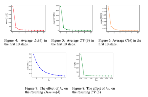
In order to determine the required number of SGD steps, the effect of [math]\displaystyle{ \lambda_s }[/math], and the importance of [math]\displaystyle{ \lambda_s }[/math] on the each losses in the cost function, the authors have tried different values of these parameters using the first example from each class of the CIFAR-10 validation set. Based on figure 4, 5, and 6, we can see that the [math]\displaystyle{ L(\delta) }[/math] (classification loss), [math]\displaystyle{ TV(\delta) }[/math] (Total Variation loss), [math]\displaystyle{ C(\delta) }[/math] (color regularizer) will converge to zero with 10 SGD steps. Note that since only 1-channel attack was used in this part of the experiment the [math]\displaystyle{ dissim(\delta) }[/math]was indeed zero. In figure 6 and 7, we can see the effect of [math]\displaystyle{ \lambda_s }[/math] on the dissimilarity loss and the effect of [math]\displaystyle{ \lambda_{tv} }[/math] on the total variation loss respectively.

Image: 500 pixels

Experiments

The authors used two experiments to prove that their approach to attack a certified model was actually able to break those defenses. The datasets used for both of these experiments were CIFAR10 and ImageNet dataset.

Attack on Randomized Smoothing

Randomized Smoothing is an adversarial defense against [math]\displaystyle{ l_\text{p} }[/math]-norm bounded attacks. The deep neural network model is trained on a randomly augmented batch of images. Perturbations are made to the original image such that they satisfy the previously defined conditions and spoof certificates are generated for an incorrect class by generating multiple adversarial images.

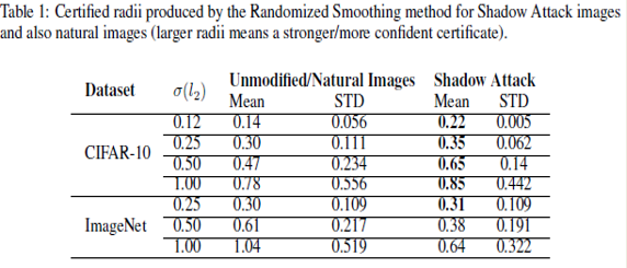
The following table shows the results of applying the 'Shadow Attack' approach to Randomized Smoothing -

Image: 600 pixels

Table 1 : Certified radii produced by the Randomized Smoothing method for Shadow Attack images and also natural images (larger radii means a stronger/more confident certificate)

The third and the fifth column correspond to the mean radius of the certified region of the original image and the mean radius of the spoof certificate of the perturbed images, respectively. It was observed that the mean radius of the certificate of adversarial images was greater than the mean radius of the original image certificate. This proves that the 'Shadow Attack' approach was successful in creating spoof certificates of greater radius and with the wrong label. This also proves that the approach used in the paper was successful in breaking the certified defenses.

Attack on CROWN-IBP

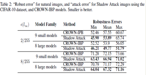
Crown IBP is an adversarial defense against [math]\displaystyle{ l_\text{inf} }[/math]-norm bounded attacks. The same approach was applied for the CROWN-IBP defense and the table below shows the results.

Image: 500 pixels

Table 2 : “Robust error” for natural images, and “attack error” for Shadow Attack images using the CIFAR-10 dataset, and CROWN-IBP models. Smaller is better.)

The above table shows the robustness errors in the case of the CROWN-IBP method and the attack images. It is seen that the errors in the case of the attack were less than the equivalent errors for CROWN-IBP, which suggests that the authors' 'Shadow Attack' approach was successful in breaking the [math]\displaystyle{ l_\text{inf} }[/math]-norm certified defenses as well.

Conclusion

From the above approach used in a couple of experiments, we can conclude that it is possible to produce adversarial examples with ‘spoofed’ certified robustness by using large-norm perturbations. The perturbations generated are smooth and natural-looking while being large enough in norm to escape the certification regions of state-of-the-art principled defenses. The major takeaway of the paper would be that the certificates produced by certifiably robust classifiers are not always good indicators of robustness or accuracy.

Critiques

It is noticeable in this paper that using the mathematical formulation of the defenses and certifications is considered a weak method, whereas the constraint is imposed by [math]\displaystyle{ l_{p} }[/math] as assumed in equation \eqref{eq:op}. The top models can not achieve certifications beyond [math]\displaystyle{ \epsilon = 0.3 }[/math] disturbance in [math]\displaystyle{ l_{2} }[/math] norm, while disturbances [math]\displaystyle{ \epsilon = 4 }[/math] added to the target input are barely noticeable by human eyes, and [math]\displaystyle{ \epsilon = 100 }[/math] , when applied to the original image are still easily classified by humans as belonging to the same class. As discussed by many authors, the perception of multi-dimensional space by human eyes goes beyond what the [math]\displaystyle{ l_{p} }[/math] norm is capable of capturing and synthesizing. It is yet to be proposed more comprehensive metrics and algorithms capable of capturing the correlation between pixels of an image or input data which can better translate to optimization algorithms how humans distinguish features of an input image. Such a metric would allow the optimization algorithms to have better intuition on the subtle variations introduced by adversaries in the input data.

References

[1] Xu, H., Ma, Y., Liu, H. C., Deb, D., Liu, H., Tang, J. L., & Jain, A. K. (2020). Adversarial Attacks and Defenses in Images, Graphs and Text: A Review. International Journal of Automation and Computing, 17(2), 151–178.

[2] Christian Szegedy,Wojciech Zaremba, Ilya Sutskever, Joan Bruna, Dumitru Erhan, Ian Goodfellow, and Rob Fergus. Intriguing properties of neural networks. arXiv preprint arXiv:1312.6199, 2013.

[3] Ali Shafahi, Mahyar Najibi, Amin Ghiasi, Zheng Xu, John Dickerson, Christoph Studer, Larry S Davis, Gavin Taylor, and Tom Goldstein. Adversarial training for free! arXiv preprint arXiv:1904.12843, 2019.

[4] Aleksander Madry, Aleksandar Makelov, Ludwig Schmidt, Dimitris Tsipras, and Adrian Vladu. Towards deep learning models resistant to adversarial attacks. arXiv preprint arXiv:1706.06083, 2017.

[5] Anish Athalye, Nicholas Carlini, and David Wagner. Obfuscated gradients give a false sense of security: Circumventing defenses to adversarial examples. arXiv preprint arXiv:1802.00420, 2018.