Graph Structure of Neural Networks: Difference between revisions
| Line 24: | Line 24: | ||
= Discussions and Conclusions = | = Discussions and Conclusions = | ||
[[File: | [[File:Result2_441_2020Group16.png]] | ||
== 1. Neural networks performance depends on its structure == | == 1. Neural networks performance depends on its structure == | ||
Revision as of 15:22, 15 November 2020
Presented By
Xiaolan Xu, Robin Wen, Yue Weng, Beizhen Chang
Introduction
We develop a new way of representing a neural network as a graph, which we call relational graph. Our key insight is to focus on message exchange, rather than just on directed data flow. As a simple example, for a fixedwidth fully-connected layer, we can represent one input channel and one output channel together as a single node, and an edge in the relational graph represents the message exchange between the two nodes (Figure 1(a)).
Relational Graph
Parameter Definition
(1) Clustering Coefficient
(2) Average Path Length
Experimental Setup (Section 4 in the paper)
Discussions and Conclusions
1. Neural networks performance depends on its structure
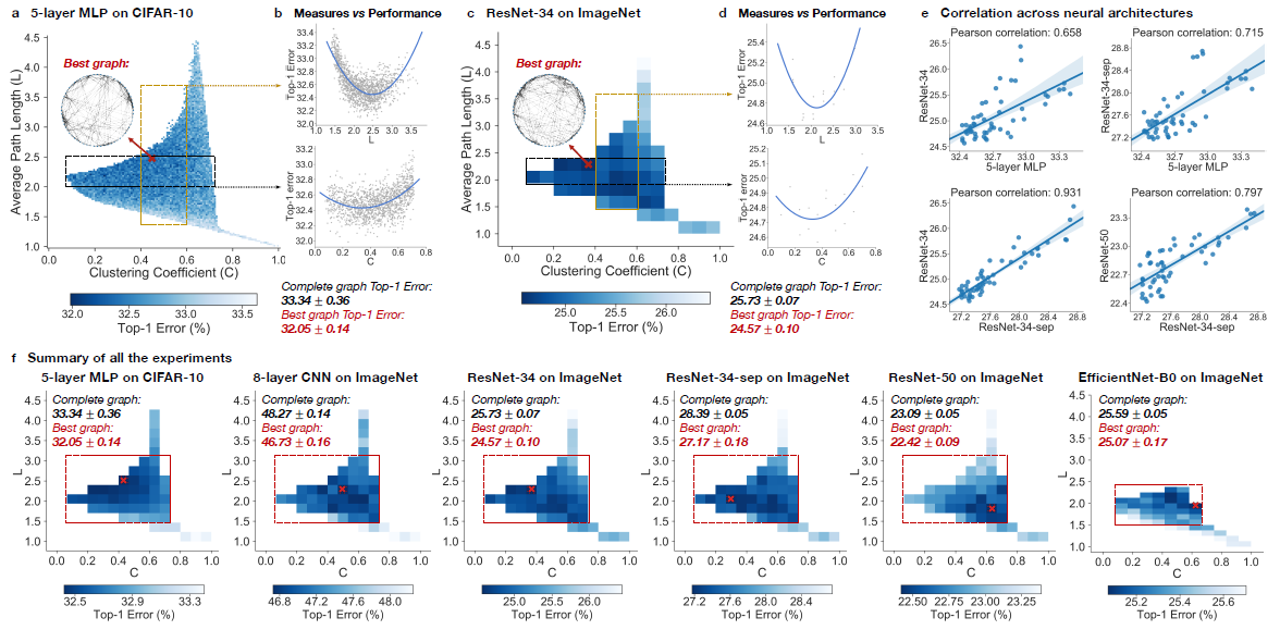
We collect top-1 errors for all the sampled relational graphs on different tasks and architectures, and also record the graph measures (average path length and clustering coefficient) for each sampled graph. The heat maps of graph measures vs. predictive performance (Figure 4(a)(c)(f)) show that there exist graph structures that can outperform the complete graph (the pixel on bottom right) baselines. The best performing relational graph can outperform the complete graph baseline by 1.4% top-1 error for MLP on CIFAR-10, and 0.5% to 1.2% for models on ImageNet. The existence of well-performing models in many different experimental setups suggests that graph structure does matter for the predictive performance of neural networks.
2. Sweet spot where performance is significantly improved
To further reduce the impact of training noise, we downsample and aggregate the 3942 graphs in Figure 4(a) into a coarse resolution of 52 bins, where each bin represents the average performance of graphs that fall into the bin, as is shown in Figure 4(f) (leftmost). With this aggregated heat map, it is clear that well-performing graphs tend to cluster into a “sweet spot”, shown in the red rectangle.
3. Relationship between neural network’s performance and parameters
In Figure 4(f), we observe that neural network’s predictive performance is approximately a smooth function of the clustering coefficient and average path length of its relational graph. Keeping one graph measure fixed (in a small range), we visualize network performances against the other measure (Shown in Figure 4(b)(d)). We use second degree polynomial regression to visualize the overall trend. We observe that both clustering coefficient and average path length are indicative of neural network performance, demonstrating a U-shape correlation
4. Consistency among many different tasks and datasets
Given that relational graph defines a shared design space across various neural architectures, we observe that relational graphs with certain graph measures may consistently perform well regardless of how they are instantiated. Qualitative consistency. We visually observe in Figure 4(f) that the region of well-performing graphs is consistent across different architectures datasets. Specifically, we found that graphs with clustering coefficient within [0.1, 0.7] and average path length within [1.5, 3] consistently outperform the baseline complete graph. Moreover, the U-shape trends between graph measures and corresponding neural network performance, shown in Figure 4(b)(d), are also visually consistent across architectures and datasets. 52 graphs: correlation = 0.90 3 epochs: correlation = 0.93 Figure 5: The correlation between findings in intermediate training epochs and the final epoch (left), and using fewer samples of relational graphs and using all the graphs (right). Quantitative consistency. To further quantify this consistency across tasks and architectures, we select the 52 bins in the heat map in Figure 4(f), where the bin value indicates the average performance of relational graphs whose graph measures fall into the bin range. We plot the correlation of the 52 bin values across different pairs of tasks, shown in Figure 4(e). We observe that the performance of relational graphs with certain graph measures correlates across different tasks and architectures. For example, even though a ResNet-34 has much higher complexity than a 5-layer MLP, and ImageNet is a much more challenging dataset than CIFAR-10, a fixed set relational graphs would perform similarly in both settings, indicated by a Pearson correlation of 0.658 (p-value < 10−8 ).
