GradientLess Descent: Difference between revisions
No edit summary |
|||
| Line 34: | Line 34: | ||
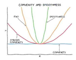
We remark that if <math display="inline">f</math> is twice continuously differentiable, this is simply equivalent to the eigenvalues of the Hessian matrix <math display="inline">\textbf{H}f</math> being bounded between <math display="inline">\alpha</math> and <math display="inline">\beta</math>. Further intuition can be gained from the image below, showing how such a function can be contained within quadratic bounds. | We remark that if <math display="inline">f</math> is twice continuously differentiable, then this is simply equivalent to the eigenvalues of the Hessian matrix <math display="inline">\textbf{H}(f)</math> being bounded between <math display="inline">\alpha</math> and <math display="inline">\beta</math>. Further intuition can be gained from the image below, showing how such a function can be contained within quadratic bounds. | ||
[[File:ConvexSmooth.PNG|frame|Relationship between convexity and smoothness.]] | [[File:ConvexSmooth.PNG|frame|Relationship between convexity and smoothness.]] | ||
In convex analysis, one usually says that a function has condition number <math display="inline">Q</math> if it is both <math display="inline">\alpha</math>-strongly convex, and <math display="inline">\beta</math>-smooth, and <math display="inline">\frac{\beta}{\alpha} \leq Q</math>. | In convex analysis, one usually says that a function has condition number <math display="inline">Q</math> if it is both <math display="inline">\alpha</math>-strongly convex, and <math display="inline">\beta</math>-smooth, and <math display="inline">\frac{\beta}{\alpha} \leq Q</math>. | ||
The authors of this paper consider the more general case where <math display="inline">f</math> is a monotone transformation of | The authors of this paper consider the more general case where <math display="inline">f</math> is a monotone transformation of an <math display="inline">\alpha</math>-strongly convex and <math display="inline">\beta</math>-smooth function; for simplicity and transparency, we shall not consider these extensions here, but shall note that their proofs are quite elementary. | ||
===Zeroth-Order Optimization=== | ===Zeroth-Order Optimization=== | ||
Revision as of 14:10, 8 November 2020
Introduction
In this presentation, we are interested in minimizing a smooth convex function without ever computing its derivatives.
Motivation and Set-up
A general optimization question can be formulated by asking to minimize an objective function [math]\displaystyle{ f : \mathbb{R}^n \to \mathbb{R} }[/math], which means finding: \begin{align*} x^* = \mathrm{argmin}_{x \in \mathbb{R}^n} f(x) \end{align*}
Depending on the nature of [math]\displaystyle{ f }[/math], different settings may be considered:
- Convex vs non-convex objective functions;
- Differentiable vs non-differentiable objective functions;
- Allowed function or gradient computations;
- Noisy/Stochastic oracle access.
For the purpose of this paper, we consider convex smooth objective noiseless functions, where we have access to function computations but not gradient computations. This class of functions is quite common in practice; for instance, they make special appearances in the reinforcement learning literature.
To be even more precise, in our context we let [math]\displaystyle{ K \subseteq \mathbb{R}^n }[/math] be compact [math]\displaystyle{ f : K \to \mathbb{R} }[/math] be [math]\displaystyle{ \beta }[/math]-smooth and [math]\displaystyle{ \alpha }[/math]-strongly convex.
Definition 1
A convex continuously differentiable function [math]\displaystyle{ f : K \to \mathbb{R} }[/math] is [math]\displaystyle{ \alpha }[/math]-strongly convex for [math]\displaystyle{ \alpha \gt 0 }[/math] if \begin{align*} f(y) \geq f(x) + \left\langle \nabla f(x), y-x\right\rangle + \frac{\alpha}{2} ||y - x||^2 \end{align*} [math]\displaystyle{ \forall x,y \in K }[/math]. It is called [math]\displaystyle{ \beta }[/math]-smooth for [math]\displaystyle{ \beta \gt 0 }[/math] if \begin{align*} f(y) \leq f(x) + \left\langle \nabla f(x), y-x\right\rangle + \frac{\beta}{2} || y - x||^2 \end{align*} [math]\displaystyle{ \forall x,y \in K }[/math]
We remark that if [math]\displaystyle{ f }[/math] is twice continuously differentiable, then this is simply equivalent to the eigenvalues of the Hessian matrix [math]\displaystyle{ \textbf{H}(f) }[/math] being bounded between [math]\displaystyle{ \alpha }[/math] and [math]\displaystyle{ \beta }[/math]. Further intuition can be gained from the image below, showing how such a function can be contained within quadratic bounds.

In convex analysis, one usually says that a function has condition number [math]\displaystyle{ Q }[/math] if it is both [math]\displaystyle{ \alpha }[/math]-strongly convex, and [math]\displaystyle{ \beta }[/math]-smooth, and [math]\displaystyle{ \frac{\beta}{\alpha} \leq Q }[/math]. The authors of this paper consider the more general case where [math]\displaystyle{ f }[/math] is a monotone transformation of an [math]\displaystyle{ \alpha }[/math]-strongly convex and [math]\displaystyle{ \beta }[/math]-smooth function; for simplicity and transparency, we shall not consider these extensions here, but shall note that their proofs are quite elementary.
Zeroth-Order Optimization
In zeroth-order optimization, we are interested in minimizing a function without computing its derivatives. This is important in many practical applications in which derivatives may not be available, or they may be difficult to compute, such as:
- Combinatorial (i.e. discrete) optimization
- Instances of non-analytic loss functions (e.g. hyperparameter tuning)
- Adversarial attacks
- Reinforcement learning
Curiously, a large amount of this approach focuses on approximating gradients and then using first-order optimization algorithms.
This paper presents a purely gradientless algorithm, proposes a geometric approach to analyze the algorithm, and proves a [math]\displaystyle{ O( k Q \log (n / \epsilon )) }[/math] convergence bound. Here the latent dimension is [math]\displaystyle{ k }[/math] and [math]\displaystyle{ k \lt n }[/math], where [math]\displaystyle{ n }[/math] is the input dimension.
GradientLess Descent Algorithm
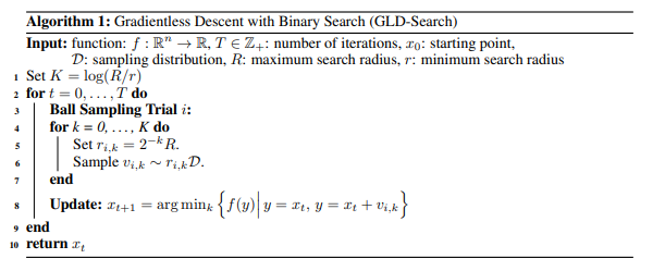
The proposed algorithm is given in the picture below.

Observe that at each step, we perform binary search over several concentric circles and randomly sample points, in the hopes that if we take a small step in a random direction this will reduce the value of the objective function.
Proof of correctness
The correctness of this algorithm hinges on two observations. The first one is about the volume of the intersection of high-dimensional balls; we call this intersection a hyperspherical cap.
Theorem 1
Let [math]\displaystyle{ B_1, B_2 \subseteq \mathbb{R}^n }[/math] be balls of radii [math]\displaystyle{ r_1, r_2 }[/math]. Let [math]\displaystyle{ \ell }[/math] be the distance between the centres. If [math]\displaystyle{ r_1 \in \left[ \frac{\ell}{2 \sqrt{n}} , \frac{\ell}{\sqrt{n}} \right] }[/math] and [math]\displaystyle{ r_2 \geq \ell - \frac{\ell}{4n} }[/math], then [math]\displaystyle{ \lambda (B_1 \cap B_2) \geq c_n \lambda (B_1) }[/math], where [math]\displaystyle{ c_n \geq \frac{1}{4} }[/math].
Using this theorem about random searches in high dimensions, we can prove the correctness of our algorithm.
Theorem 2
[math]\displaystyle{ \forall x \in K }[/math] s.t. [math]\displaystyle{ \frac{3}{5Q} ||x - x^*|| \in [C_1, C_2] }[/math], we can find integers [math]\displaystyle{ 0 \leq k_1, k_2 \lt \log \frac{C_2}{C_1} }[/math] such that if [math]\displaystyle{ r = 2^{k_1}C_1 }[/math] or [math]\displaystyle{ r = 2^{-k_2}C_2 }[/math], then a sample [math]\displaystyle{ y }[/math] from the uniform distribution on [math]\displaystyle{ B_x = B\left( x, \frac{r}{\sqrt{n}} \right) }[/math] satisfies \begin{align*} f(y) - f(x^*) \leq (f(x) - f(x^*)) \left( 1- \frac{1}{5nQ} \right) \end{align*} with probability at least [math]\displaystyle{ \frac{1}{4} }[/math].
Notice how the second theorem implies that with a quarter probability, [math]\displaystyle{ f(y) }[/math] is closer to the optimum,[math]\displaystyle{ f(x^*), }[/math] than [math]\displaystyle{ f(x) }[/math] is.
For proofs of these theorems, please watch my talk.
Results
We compare the GradientLess Descent algorithm to a benchmark established by the Augmented Randomized Search algorithm proposed in 2011.
For this comparison, we defined the function [math]\displaystyle{ f(x) = \frac{1}{2} x^T H x }[/math] where [math]\displaystyle{ H }[/math] is a diagonal matrix with eigenvalues linearly interpolating the interval [math]\displaystyle{ [\alpha , \beta] }[/math]. We observe that in most scenarios, GradientLess Descent beats the benchmark.
Conclusion
This research paper has analyzed a randomized algorithm where a search direction is sampled from the standard Gaussian. This is a direct search-based algorithm, which yields the convergence rate that is polylogarithmically dependent on dimensionality for any monotone transform of a smooth and strongly convex objective with a low-dimensional structure. In this algorithm, the step-size is considered as an approximate line to search all the possible values of a grid spanning an interval with uniform spacing on a log-scale. They show a geometric decrease of the function value regret, up to a constant defined by the minimum step-size, on strongly convex functions with Lipschitz smooth gradient.\\
Critiques
Although the theoretical guarantees presented in the paper are interesting, this is not clear how this algorithm is applicable in practice. This is because this paper assumes we do not have access to the objective function, and they are only able to use function evaluations. Besides, there is a strong assumption that the function is smooth and strongly convex. Considering this, my main concern is how we can make sure the objective function is smooth and strongly convex while we do not have access to it explicitly? (if we have explicit access to the function and this is smooth and strongly convex, why shouldn't we use gradient based methods?!) Further, what happens if the objective function violates the smooth and strongly convex condition? Can we still employ this algorithm?
Bibliography
1. Daniel Golovin et al. Gradientless descent: High-dimensional zeroth-order optimization". In: arXiv preprint arXiv:1911.06317 (2019).
2. Shengqiao Li. Concise formulas for the area and volume of a hyperspherical cap". In: Asian Journal of Mathematics and Statistics 4.1 (2011), pp. 66-70.
3. Yurii Nesterov and Vladimir Spokoiny. Random gradient-free minimization of convex functions. In: Foundations of Computational Mathematics 17.2 (2017), pp. 527-566.
4. R Tyrrell Rockafellar. Convex analysis. 28. Princeton university press, 1970.
