User:Yktan: Difference between revisions
| Line 57: | Line 57: | ||
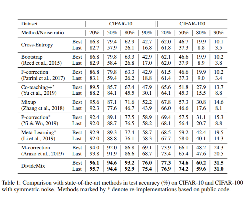
[[File: | [[File:divideMixtable1.PNG | center]] | ||
From table1, we notice that none of these methods can consistently outperform others across different datasets. M-correction excels at symmetric noise, whereas Meta-Learning performs better for asymmetric noise. DivideMix outperforms state-of-the-art methods by a large margin across all noise ratios. DivideMix outperforms state-of-the-art methods by a large margin across all noise ratios. The improvement is substantial (∼10% in accuracy) for the more challenging CIFAR-100 with high noise ratios. | From table1, we notice that none of these methods can consistently outperform others across different datasets. M-correction excels at symmetric noise, whereas Meta-Learning performs better for asymmetric noise. DivideMix outperforms state-of-the-art methods by a large margin across all noise ratios. DivideMix outperforms state-of-the-art methods by a large margin across all noise ratios. The improvement is substantial (∼10% in accuracy) for the more challenging CIFAR-100 with high noise ratios. | ||
Revision as of 14:32, 3 November 2020
Presented by
Ruixian Chin, Yan Kai Tan, Jason Ong, Wen Cheen Chiew
Introduction
Motivation
Model Architecture
DivideMix leverages semi-supervised learning to achieve effective modelling. The sample is first split into a labelled set and an unlabeled set. This is achieved by fitting a Gaussian Mixture Model as a per-sample loss distribution. The unlabeled set is made up of data points with discarded labels deemed noisy. Then, to avoid confirmation bias, which is typical when a model is self-training, two models are being trained simultaneously to filter error for each other. This is done by dividing the data using one model and then training the other model. This algorithm, known as Co-divide, keeps the two networks from converging when training, which avoids the bias from occurring. Figure 1 describes the algorithm in graphical form.

For each epoch, the network divides the dataset into a labelled set consisting of clean data, and an unlabeled set consisting of noisy data, which is then used as training data for the other network, where training is done in mini-batches. For each batch of the labelled samples, co-refinement is performed by using the ground truth label [math]\displaystyle{ y_b }[/math], the predicted label [math]\displaystyle{ p_b }[/math], and the posterior is used as the weight, [math]\displaystyle{ w_b }[/math].
Then, a sharpening function is implemented on this weighted sum to produce the estimate, [math]\displaystyle{ \hat{y}_b }[/math]. Using all these predicted labels, the unlabeled samples will then be assigned a "co-guessed" label, which should produce a more accurate prediction. Having calculated all these labels, MixMatch is applied to the combined mini-batch of labeled, [math]\displaystyle{ \hat{X} }[/math] and unlabeled data, [math]\displaystyle{ \hat{U} }[/math], where, for a pair of samples and their labels, one new sample and new label is produced. More specifically, for a pair of samples [math]\displaystyle{ (x_1,x_2) }[/math] and their labels [math]\displaystyle{ (p_1,p_2) }[/math], the mixed sample [math]\displaystyle{ (x',p') }[/math] is:
[math]\displaystyle{ \begin{alignat}{2} \lambda &\sim Beta(\alpha, \alpha) \\ \lambda ' &= max(\lambda, 1 - \lambda) \\ x' &= \lambda ' x_1 + (1 - \lambda ' ) x_2 \\ p' &= \lambda ' p_1 + (1 - \lambda ' ) p_2 \\ \end{alignat} }[/math]
MixMatch transforms [math]\displaystyle{ \hat{X} }[/math] and [math]\displaystyle{ \hat{U} }[/math] into [math]\displaystyle{ X' }[/math] and [math]\displaystyle{ U' }[/math]. Then, the loss on [math]\displaystyle{ X' }[/math], [math]\displaystyle{ L_X }[/math] (Cross-entropy loss) and the loss on [math]\displaystyle{ U' }[/math], [math]\displaystyle{ L_U }[/math] (Mean Squared Error) are calculated. A regularization term, [math]\displaystyle{ L_{reg} }[/math], is introduced to regularize the model's average output across all samples in the mini-batch. Then, the total loss is calculated as:
,
where [math]\displaystyle{ \lambda_r }[/math] is set to 1, and [math]\displaystyle{ \lambda_u }[/math] is used to control the unsupervised loss.
Lastly, the stochastic gradient descent formula is updated with the calculated loss, [math]\displaystyle{ L }[/math], and the estimated parameters, [math]\displaystyle{ \boldsymbol{ \theta } }[/math].
Results
Applications: There are four datasets: CIFAR-10, CIFAR100 (Krizhevsky & Hinton, 2009)(both contain 50K training images and 10K test images of size 32 × 32), Clothing1M (Xiao et al., 2015), and WebVision (Li et al., 2017a). We experiment with two types of label noise: symmetric and asymmetric. We use an 18-layer PreAct Resnet (He et al., 2016) and train it using SGD with a momentum of 0.9, a weight decay of 0.0005, and a batch size of 128. The network is trained for 300 epochs. We set the initial learning rate as 0.02, and reduce it by a factor of 10 after 150 epochs. The warm-up period is 10 epochs for CIFAR-10 and 30 epochs for CIFAR-100. For all CIFAR experiments, we use the same hyperparameters M = 2, T = 0.5, and α = 4. τ is set as 0.5 except for 90% noise ratio when it is set as 0.6.
Comparison of State-of-the-Art Methods The effectiveness of DivideMix was shown by comparing the test accuracy with the most recent state-of-the-art methods: Meta-Learning (Li et al., 2019) proposes a gradient-based method to find model parameters that are more noise-tolerant; Joint-Optim (Tanaka et al., 2018) and P-correction (Yi & Wu, 2019) jointly optimize the sample labels and the network parameters; M-correction (Arazo et al., 2019) models sample loss with BMM and apply MixUp. The following are the results on CIFAR-10 and CIFAR-100 with different levels of symmetric label noise ranging from 20% to 90%. We report both the best test accuracy across all epochs and the averaged test accuracy over the last 10 epochs.

From table1, we notice that none of these methods can consistently outperform others across different datasets. M-correction excels at symmetric noise, whereas Meta-Learning performs better for asymmetric noise. DivideMix outperforms state-of-the-art methods by a large margin across all noise ratios. DivideMix outperforms state-of-the-art methods by a large margin across all noise ratios. The improvement is substantial (∼10% in accuracy) for the more challenging CIFAR-100 with high noise ratios.
DivideMix was compared with the state-of-the-art methods with the other two datasets: Clothing1M and WebVision. It also shows that DivideMix consistently outperforms state-of-the-art methods across all datasets with different types of label noise. For WebVision, DivideMix achieves more than 12% improvement in top-1 accuracy.
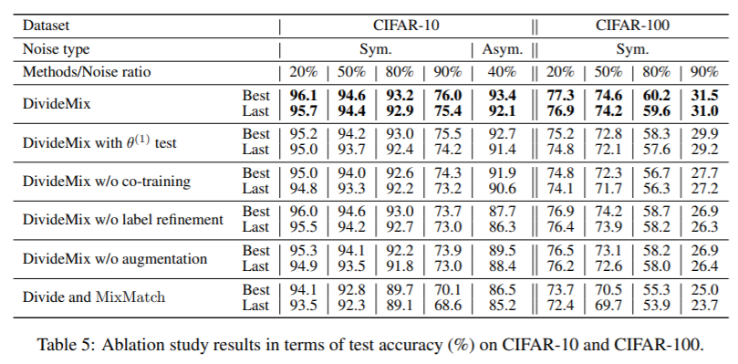
Ablation Study The effect of removing different components to provide insights into what makes DivideMix successful. We analyze the results in Table 5 as follows.

We find that both label refinement and input augmentation are beneficial for DivideMix.