GradientLess Descent: Difference between revisions
No edit summary |
|||
| Line 34: | Line 34: | ||
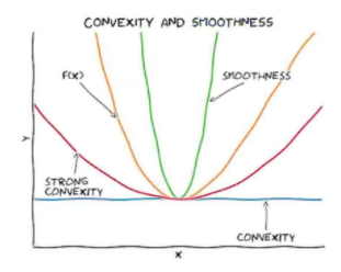
We remark that if <math display="inline">f</math> is twice continuously differentiable, this is simply equivalent to the eigenvalues of the Hessian matrix <math display="inline">Hf</math> being bounded between <math display="inline">\alpha</math> and <math display="inline">\beta</math>. Further intuition can be gained from the image below, showing how such a function can be contained within quadratic bounds: | We remark that if <math display="inline">f</math> is twice continuously differentiable, this is simply equivalent to the eigenvalues of the Hessian matrix <math display="inline">Hf</math> being bounded between <math display="inline">\alpha</math> and <math display="inline">\beta</math>. Further intuition can be gained from the image below, showing how such a function can be contained within quadratic bounds: | ||
[[File:ConvexSmooth.PNG| | [[File:ConvexSmooth.PNG|frame|Relationship between convexity and smoothness.]] | ||
===Zeroth-Order Optimisation=== | ===Zeroth-Order Optimisation=== | ||
Revision as of 18:21, 31 October 2020
Introduction
Motivation and Set-up
A general optimisation question can be formulated by asking to minimise an objective function [math]\displaystyle{ f : \mathbb{R}^n \to \mathbb{R} }[/math], which means finding: \begin{align*} x^* = \mathrm{argmin}_{x \in \mathbb{R}^n} f(x) \end{align*}
Depending on the nature of [math]\displaystyle{ f }[/math], different settings may be considered:
- Convex vs non-convex objective functions;
- Differentiable vs non-differentiable objective functions;
- Allowed function or gradient computations;
- Noisy/Stochastic oracle access.
For the purpose of this paper, we consider convex smooth objective noiseless functions, where we have access to function computations but not gradient computations. This class of functions is quite common in practice; for instance, they make special appearances in the reinforcement learning literature.
To be even more precise, in our context we let [math]\displaystyle{ K \subseteq \mathbb{R}^n }[/math] be compact [math]\displaystyle{ f : K \to \mathbb{R} }[/math] be [math]\displaystyle{ \beta }[/math]-smooth and [math]\displaystyle{ \alpha }[/math]-strongly convex.
Definition 1
A convex continuously differentiable function [math]\displaystyle{ f : K \to \mathbb{R} }[/math] is [math]\displaystyle{ \alpha }[/math]-strongly convex for [math]\displaystyle{ \alpha \gt 0 }[/math] if \begin{align*} f(y) \geq f(x) + \left\langle \nabla f(x), y-x\right\rangle + \frac{\alpha}{2} ||y - x||^2 \end{align*} for all [math]\displaystyle{ x,y \in K }[/math]. It is called [math]\displaystyle{ \beta }[/math]-smooth for [math]\displaystyle{ \beta \gt 0 }[/math] if \begin{align*} f(y) \leq f(x) + \left\langle \nabla f(x), y-x\right\rangle + \frac{\beta}{2} || y - x||^2 \end{align*} for all [math]\displaystyle{ x,y \in K }[/math]
We remark that if [math]\displaystyle{ f }[/math] is twice continuously differentiable, this is simply equivalent to the eigenvalues of the Hessian matrix [math]\displaystyle{ Hf }[/math] being bounded between [math]\displaystyle{ \alpha }[/math] and [math]\displaystyle{ \beta }[/math]. Further intuition can be gained from the image below, showing how such a function can be contained within quadratic bounds:
