XGBoost: A Scalable Tree Boosting System

Presented by

• Qianying Zhao
• Hui Huang
• Lingyun Yi
• Jiayue Zhang
• Siao Chen
• Rongrong Su
• Gezhou Zhang
• Meiyu Zhou

2 Tree Boosting In A Nutshell

2.1 Regularized Learning Objective

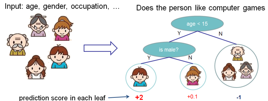
1. Regression Decision Tree (also known as classification and regression tree):

• Decision rules are the same as in decision tree
• Contains one score in each leaf value

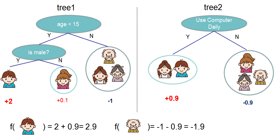
2. Model and Parameter

Model: Assuming there are K trees [math]\displaystyle{ \hat y_i = \sum^K_{k=1} f_k(x_I), f_k \in Ƒ }[/math]

Object: [math]\displaystyle{ Obj = \sum_{i=1}^n l(y_i,\hat y_i)+\sum^K_{k=1}\omega(f_k) }[/math]

where [math]\displaystyle{ \sum^n_{i=1}l(y_i,\hat y_i) }[/math] is training loss, [math]\displaystyle{ \sum_{k=1}^K \omega(f_k) }[/math] is complexity of Trees

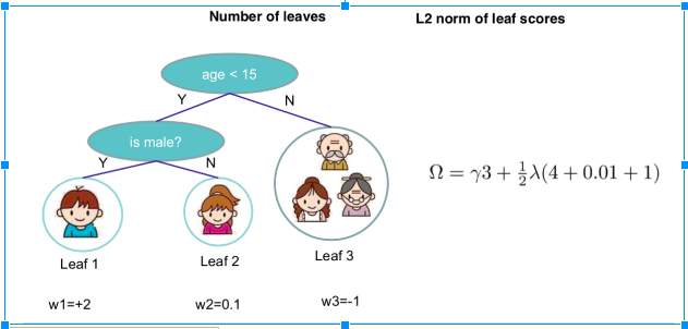
So the target function that needed to optimize is:[math]\displaystyle{ \sum_{i=1}^n l(y_i,\hat y_i)+\sum^K_{k=1}\omega(f_k), f_k \in Ƒ }[/math], where [math]\displaystyle{ \omega(f) = \gamma T+\frac{1}{2}\lambda||w||^2 }[/math]

For example:

Let's look at [math]\displaystyle{ \hat y_i }[/math]

[math]\displaystyle{ \hat y{i}^{(0)} = 0 }[/math]

[math]\displaystyle{ \hat y{i}^{(1)} = f_1(x_i)=\hat y_i^{(0)}+f_1(x_i) }[/math]

[math]\displaystyle{ \hat y{i}^{(2)} = f_1(x_i) + f_2(x_i)=\hat y_i^{(1)}+f_2(x_i) }[/math]

...

[math]\displaystyle{ \hat y{i}^{(t)} = \sum^t_{i=1}f_k(x_i)=\hat y_i^{(t-1)}+f_t(x_i) }[/math]

So [math]\displaystyle{ Obj^{(t)} = \sum_{i=1}^n l(y_i,\hat y_i^{(t)})+\sum^t_{i=1}\omega(f_i) }[/math]

                              =[math]\displaystyle{ \sum_{i=1}^n l(y_i,\hat y_i^{(t-1)}+f_t(x_i))+omega(f_t)+constant }[/math]

Take Taylor Expansion of the objective

[math]\displaystyle{ f(x+\delta x) \simeq f(x)+f^{'}(x)\delta x+\frac{1}{2}f^{''}(x)\delta x^2 }[/math]

then

[math]\displaystyle{ Obj^{(t)} = \sum^n_{i=1}[l(y_i,\hat y_i^{(t-1)})+g_if_t(x_i)+\frac{1}{2}h_i(x_i)]+\omega(f_t)+constant }[/math]

where [math]\displaystyle{ g_i =ə_{(\hat y_i)^{(t-1)}}(\hat y_i^{(t-1)}-y_i)^2 = 2(\hat y_i^{(t-1)}-y_i)h_i = ə^2_{(\hat y_i)^{(t-1)}}(\hat y_i^{t-1)}-y_i)^2 =2 }[/math]

Define [math]\displaystyle{ I_j={i|q(x_i)=j} }[/math] as the instance set of leaf j and [math]\displaystyle{ f_t(x_i)=w_j }[/math]. We can rewrite target function as follows

[math]\displaystyle{ Obj^{(t)} = \sum^{T}_{j=1}[(\sum_{i\in I_j} g_i)w_{j}+\frac{1}{2}(\sum_{i\in I_j}h_i + \lambda)w_j^2]+\gamma T }[/math]

The optimal weight [math]\displaystyle{ w^*_j }[/math] of node j is [math]\displaystyle{ w_j^*=\frac{\sum_{i\in I_j}g_i}{\sum_{i\in I_j}h_i+\lambda} }[/math]

The loss reduction after the split is given by

[math]\displaystyle{ Obj_{split}=\frac{1}{2}[\frac{(\sum_{i \in I_l} g_i)^2}{\sum_{i \in I_l} h_i+\lambda}+\frac{(\sum_{i \in I_R} g_i)^2}{\sum_{i \in I_R} h_i+\lambda}-\frac{(\sum_{i \in I} g_i)^2}{\sum_{i \in I} h_i+\lambda}]-\lambda }[/math]

3 Split Finding Algorithms

3.1 Exact Greedy Algorithm

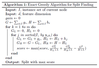
Exact greedy algorithm is a split finding algorithm enumerates over all the possible splits on all the features. However, it is impossible to efficiently do so when the data does not fit entirely into memory.

The algorithm is following:

3.2 Approximate Algorithm

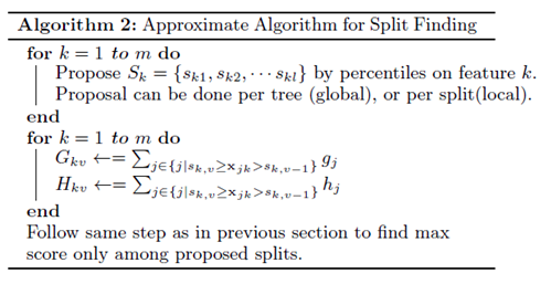
Due to limit computational memory and efficiency, the paper gives an approximate algorithm. The algorithm first proposes candidate splitting points according to percentiles of feature distribution, then it maps the continuous features into buckets split by these candidate points, aggregates the statistics and finds the best solution among proposals based on the aggregated statistics.

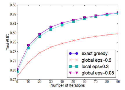
The global variant proposes all the candidate splits during the initial phase of tree construction, and uses the same proposals for split finding at all levels. The local variant re-proposes after each split.

From the figure above, the quantile strategy can get the same accuracy as exact greedy given reasonable approximation level.

3.3 Weighted Quantile Sketch

Data set splitting is one of the most important phase in the approximate algorithm. The most common approach is to split by feature’s percentile in order to obtain an uniform distribution of the selected data.

Formal, if we have the set

[math]\displaystyle{ D_k={(x_{1k},h_1),(x_{2k},h_2),...,(x_{nk},h_n)} }[/math]

We can use the following function to rank:

[math]\displaystyle{ R_k(z) = \frac{1}{\sum_{(x,h) \in D_k} h} \sum_{(x,h) \in D_k, x\lt z} h, }[/math]

The objective is to search for split points {s_{k1}, s_{k2}, …, s_{kl}} such that

[math]\displaystyle{ |r_k(s_{k,j}) – r_k(s_{k,j+1})| \lt \epsilon, }[/math]

Where [math]\displaystyle{ \epsilon }[/math] is an approximation factor. In general, it should approximately have [math]\displaystyle{ \frac{1}{\epsilon} }[/math] splitting points.

3.4 Sparsity-aware Split Finding

In real life, the input x may often be quite sparse. Possible causes are:

1. Data set contains missing values

2. Large amount of zero entries

3. Artifacts of feature engineering (ex. One-hot encoding)

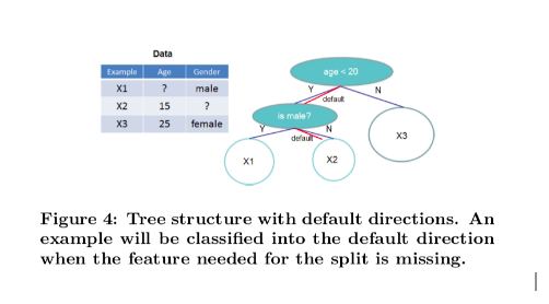
In order to solve the sparsity behavior in the data, it is proposed to create a default direction in each tree node, as shown below:

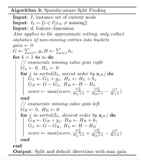
When a value in a tree node is missing, we can use the following algorithm to calculate the optimal direction to proceed:

This algorithm is also applicable to the situation where user can set a limit on the accepted value, and neglect the out-of-range value when calculating the score.

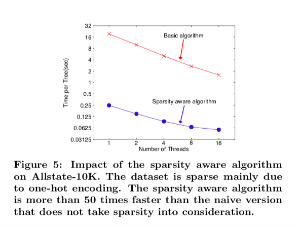
The figure below shows the result of the comparison between a basic implementation and the sparsity aware algorithm on a Allstate-10K dataset.

We can see that the sparsity aware algorithm performs 50 times better than the simple implementation.

4 System Design

4.1 Column Block for Parallel Learning

Generally, the most time-consuming part of tree learning is to get a sorted data. In XGBoost, data is stored in in-memory units, called Block.

Each column represents a feature and is sorted by the feature value.

In exact greedy algorithm, the entire dataset is stored in a single block. So, a single scan over the block will provide us the statistics needed for splitting.

   	d = maximum depth of the tree

   	K = total number of trees

   	Original spase aware algorithm costs

   	Tree boosting on block structure costs

For Approximate algorithm, the dataset can be stored in multiple blocks. Each block contains a subset of tuples in the dataset. The blocks are also in sorted order, so for the quantile finding step, a linear scan over the sorted column is enough.

   	q = number of proposal candidates in the dataset

   	B = maximum number of rows in each block

   	Original approximate algorithm with binary search costs

   	Approximate algorithm with block structure costs

4.2 Cache-aware Access

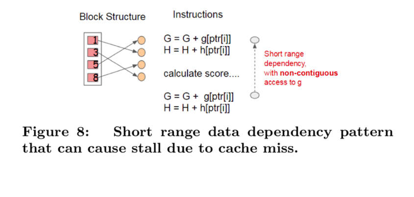
A naïve implementation of split enumeration brings in immediate read/write dependency between the accumulation and the non-continuous memory fetch operation.

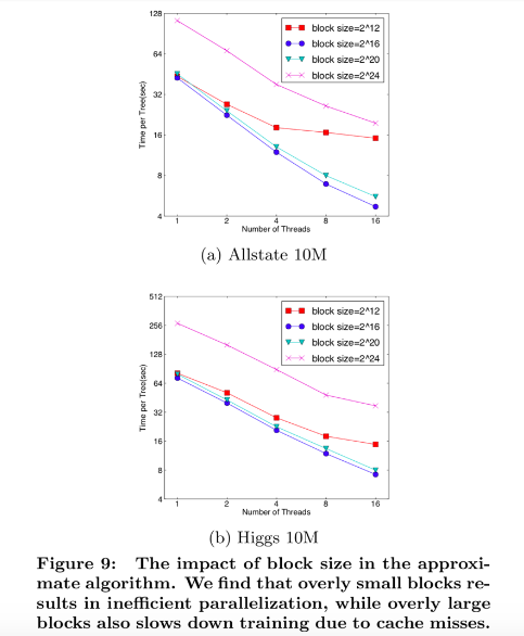
To overcome this issue in exact greedy algorithm, a cache-aware prefetching algorithm with an internal buffer allocated for fetching the gradient statistics is proposed. For approximate algorithm, since multiple blocks are used for storing the dataset, choosing the correct block size is the key.

An overly small block size results in small workload and inefficient parallelization

· An overly large block size results in cache misses as the gradient statistics do not fit into the CPU cache

Through experiment, block size of 216 balances the cache property and parallelization.

For large size dataset, data might not be fitted into main memory and has to be stored in disk space. So, enabling out-of-core computation is important for achieving scalable learning. It is ideal to have computation run in concurrence with disk reading to reduce the overhead. Two major techniques used to improve the out-of-core computation are shown below:

1) Block Compression

• Compress feature value in each block

• Decompress feature value through the thread

• Compress ratio: 26~29%

2) Block Sharding

• When multiple disks are available

• Shard the dataset onto multiple disks in an alternative manner

• Each disk has a pre-fetcher thread to fetch data into an in-memory buffer

• Training-thread alternatively reads data from each buffer