stat841F18/: Difference between revisions
| Line 31: | Line 31: | ||
== Model Architecture == | == Model Architecture == | ||
The extreme learning machine (ELM) is a particular kind of machine learning setup in which a single layer or multiple layers apply. The ELM includes numbers of hidden neurons where the input weights are assigned randomly. Extreme learning machines use the concept of random projection and early perceptron models to do specific kinds of problem-solving. | |||
==Algorithms== | |||
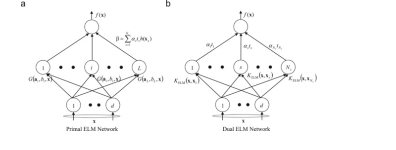
Given a single hidden layer of ELM, suppose that the output function of the <math>i</math>-th hidden node is <math>h_i(\mathbf{x})=G(\mathbf{a}_i,b_i,\mathbf{x})</math>, where <math>\mathbf{a}_i</math> and <math>b_i</math> are the parameters of the <math>i</math>-th hidden node. The output function of the ELM for SLFNs with <math>L</math> hidden nodes is: | |||
<math>f_L({\bf x})=\sum_{i=1}^L{\boldsymbol \beta}_ih_i({\bf x})</math>, where <math>{\boldsymbol \beta}_i</math> is the output weight of the <math>i</math>-th hidden node. | |||
<math>\mathbf{h}(\mathbf{x})=[G(h_i(\mathbf{x}),...,h_L(\mathbf{x}))]</math> is the hidden layer output mapping of ELM. Given <math>N</math> training samples, the hidden layer output matrix <math>\mathbf{H}</math> of ELM is given as: <math>{\bf H}=\left[\begin{matrix} | |||
{\bf h}({\bf x}_1)\\ | |||
\vdots\\ | |||
{\bf h}({\bf x}_N) | |||
\end{matrix}\right]=\left[\begin{matrix} | |||
G({\bf a}_1, b_1, {\bf x}_1) &\cdots & G({\bf a}_L, b_L, {\bf x}_1)\\ | |||
\vdots &\vdots&\vdots\\ | |||
G({\bf a}_1, b_1, {\bf x}_N) &\cdots & G({\bf a}_L, b_L, {\bf x}_N) | |||
\end{matrix}\right] | |||
</math> | |||
and <math>\mathbf{T}</math> is the training data target matrix: <math>{\bf T}=\left[\begin{matrix} | |||
{\bf t}_1\\ | |||
\vdots\\ | |||
{\bf t}_N | |||
\end{matrix}\right] | |||
</math> | |||
General speaking, ELM is a kind of regularization neural networks but with non-tuned hidden layer mappings (formed by either random hidden nodes, kernels or other implementations), its objective function is: | |||
<math> | |||
\text{Minimize: } \|{\boldsymbol \beta}\|_p^{\sigma_1}+C\|{\bf H}{\boldsymbol \beta}-{\bf T}\|_q^{\sigma_2} | |||
</math> | |||
where <math>\sigma_1>0, \sigma_2>0, p,q=0, \frac{1}{2}, 1, 2, \cdots, +\infty</math>. | |||
Different combinations of <math>\sigma_1</math>, <math>\sigma_2</math>, <math>p</math> and <math>q</math> can be used and result in different learning algorithms for regression, classification, sparse coding, compression, feature learning and clustering. | |||
As a special case, a simplest ELM training algorithm learns a model of the form (for single hidden layer sigmoid neural networks): | |||
:<math>\mathbf{\hat{Y}} = \mathbf{W}_2 \sigma(\mathbf{W}_1 x)</math> | |||
where {{math|'''W'''<sub>1</sub>}} is the matrix of input-to-hidden-layer weights, <math>\sigma</math> is an activation function, and {{math|'''W'''<sub>2</sub>}} is the matrix of hidden-to-output-layer weights. The algorithm proceeds as follows: | |||
# Fill {{math|'''W'''<sub>1</sub>}} with random values (e.g, [[Gaussian noise|Gaussian random noise]]); | |||
# estimate {{math|'''W'''<sub>2</sub>}} by [[least-squares fit]] to a matrix of response variables {{math|'''Y'''}}, computed using the [[Moore–Penrose pseudoinverse|pseudoinverse]] {{math|⋅<sup>+</sup>}}, given a [[design matrix]] {{math|'''X'''}}: | |||
#:<math>\mathbf{W}_2 = \sigma(\mathbf{W}_1 \mathbf{X})^+ \mathbf{Y}</math> | |||
<center> | <center> | ||
[[File:aa.png|800px]] | [[File:aa.png|800px]] | ||
Revision as of 00:19, 9 November 2018
Presented by
Yan Yu Chen, Qisi Deng, Hengxin Li, Bochao Zhang
Introduction
In the past two decades, due to their surprising classi- fication capability, support vector machine (SVM) [1] and its variants [2]–[4] have been extensively used in classification applications. Least square support vector machine (LS-SVM) and proximal sup- port vector machine (PSVM) have been widely used in binary classification applications. The conventional LS-SVM and PSVM cannot be used in regression and multiclass classification appli- cations directly, although variants of LS-SVM and PSVM have been proposed to handle such cases.
Motivation
There are several issues on BP learning algorithms:
(1) When the learning rate Z is too small, the learning algorithm converges very slowly. However, when Z is too large, the algorithm becomes unstable and diverges.
(2) Another peculiarity of the error surface that impacts the performance of the BP learning algorithm is the presence of local minima [6]. It is undesirable that the learning algorithm stops at a local minima if it is located far above a global minima.
(3) Neural network may be over-trained by using BP algorithms and obtain worse generalization performance. Thus, validation and suitable stopping methods are required in the cost function minimization procedure.
(4) Gradient-based learning is very time-consuming in most applications.
Due to the simplicity of their implementations, least square support vector machine (LS-SVM) and proximal support vector machine (PSVM) have been widely used in binary classification applications. The conventional LS-SVM and PSVM cannot be used in regression and multiclass classification applications directly, although variants of LS-SVM and PSVM have been proposed to handle such cases. This paper shows that both LS-SVM and PSVM can be simplified further and a unified learning framework of LS-SVM, PSVM, and other regularization algorithms referred to extreme learning machine (ELM) can be built.
Previous Work
As the training of SVMs involves a quadratic programming problem, the computational complexity of SVM training al- gorithms is usually intensive, which is at least quadratic with respect to the number of training examples
Least square SVM (LS-SVM) [2] and proximal SVM (PSVM) [3] provide fast implementations of the traditional SVM. Both LS-SVM and PSVM use equality optimization constraints instead of inequalities from the traditional SVM, which results in a direct least square solution by avoiding quadratic programming.
SVM, LS-SVM, and PSVM are originally proposed for bi- nary classification. Different methods have been proposed in or- der for them to be applied in multiclass classification problems. One-against-all (OAA) and one-against-one (OAO) methods are mainly used in the implementation of SVM in multiclass classification applications [8].
extreme learning machine (ELM) for single hidden layer feedforward neural networks (SLFNs) which randomly chooses the input weights and analytically determines the output weights of SLFNs. In theory, this algorithm tends to provide the best generalization performance at extremely fast learning speed. The experimental results based on real world benchmarking function approximation and classification problems including large complex applications show that the new algorithm can produce best generalization performance in some cases and can learn much faster than traditional popular learning algorithms for feedforward neural networks.
Model Architecture
The extreme learning machine (ELM) is a particular kind of machine learning setup in which a single layer or multiple layers apply. The ELM includes numbers of hidden neurons where the input weights are assigned randomly. Extreme learning machines use the concept of random projection and early perceptron models to do specific kinds of problem-solving.
Algorithms
Given a single hidden layer of ELM, suppose that the output function of the [math]\displaystyle{ i }[/math]-th hidden node is [math]\displaystyle{ h_i(\mathbf{x})=G(\mathbf{a}_i,b_i,\mathbf{x}) }[/math], where [math]\displaystyle{ \mathbf{a}_i }[/math] and [math]\displaystyle{ b_i }[/math] are the parameters of the [math]\displaystyle{ i }[/math]-th hidden node. The output function of the ELM for SLFNs with [math]\displaystyle{ L }[/math] hidden nodes is:
[math]\displaystyle{ f_L({\bf x})=\sum_{i=1}^L{\boldsymbol \beta}_ih_i({\bf x}) }[/math], where [math]\displaystyle{ {\boldsymbol \beta}_i }[/math] is the output weight of the [math]\displaystyle{ i }[/math]-th hidden node.
[math]\displaystyle{ \mathbf{h}(\mathbf{x})=[G(h_i(\mathbf{x}),...,h_L(\mathbf{x}))] }[/math] is the hidden layer output mapping of ELM. Given [math]\displaystyle{ N }[/math] training samples, the hidden layer output matrix [math]\displaystyle{ \mathbf{H} }[/math] of ELM is given as: [math]\displaystyle{ {\bf H}=\left[\begin{matrix} {\bf h}({\bf x}_1)\\ \vdots\\ {\bf h}({\bf x}_N) \end{matrix}\right]=\left[\begin{matrix} G({\bf a}_1, b_1, {\bf x}_1) &\cdots & G({\bf a}_L, b_L, {\bf x}_1)\\ \vdots &\vdots&\vdots\\ G({\bf a}_1, b_1, {\bf x}_N) &\cdots & G({\bf a}_L, b_L, {\bf x}_N) \end{matrix}\right] }[/math]
and [math]\displaystyle{ \mathbf{T} }[/math] is the training data target matrix: [math]\displaystyle{ {\bf T}=\left[\begin{matrix} {\bf t}_1\\ \vdots\\ {\bf t}_N \end{matrix}\right] }[/math]
General speaking, ELM is a kind of regularization neural networks but with non-tuned hidden layer mappings (formed by either random hidden nodes, kernels or other implementations), its objective function is:
[math]\displaystyle{ \text{Minimize: } \|{\boldsymbol \beta}\|_p^{\sigma_1}+C\|{\bf H}{\boldsymbol \beta}-{\bf T}\|_q^{\sigma_2} }[/math]
where [math]\displaystyle{ \sigma_1\gt 0, \sigma_2\gt 0, p,q=0, \frac{1}{2}, 1, 2, \cdots, +\infty }[/math].
Different combinations of [math]\displaystyle{ \sigma_1 }[/math], [math]\displaystyle{ \sigma_2 }[/math], [math]\displaystyle{ p }[/math] and [math]\displaystyle{ q }[/math] can be used and result in different learning algorithms for regression, classification, sparse coding, compression, feature learning and clustering.
As a special case, a simplest ELM training algorithm learns a model of the form (for single hidden layer sigmoid neural networks):
- [math]\displaystyle{ \mathbf{\hat{Y}} = \mathbf{W}_2 \sigma(\mathbf{W}_1 x) }[/math]
where Template:math is the matrix of input-to-hidden-layer weights, [math]\displaystyle{ \sigma }[/math] is an activation function, and Template:math is the matrix of hidden-to-output-layer weights. The algorithm proceeds as follows:
- Fill Template:math with random values (e.g, Gaussian random noise);
- estimate Template:math by least-squares fit to a matrix of response variables Template:math, computed using the pseudoinverse Template:math, given a design matrix Template:math:
- [math]\displaystyle{ \mathbf{W}_2 = \sigma(\mathbf{W}_1 \mathbf{X})^+ \mathbf{Y} }[/math]
Performance Verification
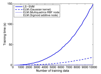
Fig. 1.
Fig. 1 shows the scalability of different classifiers: An example on letter data set. training time spent by LS-SVM and ELM (Gaussian kernel) increases sharply when the number of training data increases. However, the training time spent by ELM with Sigmoid additive node and multiquadric function node increases very slowly when the number of training data increases.
Conclusion
Critiques
References
- [1]G.-B. Huang, Q.-Y. Zhu, and C.-K. Siew, “Extreme learning machine: A new learning scheme of feedforward neural networks,” in Proc. IJCNN,Budapest, Hungary, Jul. 25–29, 2004, vol. 2, pp. 985–990.
- [2]G.-B. Huang, X.Ding, and H.Zhou, Optimization method based extreme learning machine for classification," Neurocomputing, vol. 74, no. 1-3, pp. 155-163, Dec. 2010.


