stat946w18/Wavelet Pooling For Convolutional Neural Networks

Wavelet Pooling For Convolutional Neural Networks

Your feedback on presentations

Introduction, Important Terms and Brief Summary

This paper focuses on the following important techniques:

1) Convolutional Neural Nets (CNN): These are networks with layered structures that conform to the shape of inputs and consistently obtain high accuracies in the classification of images and objects. Researchers continue to focus on CNN to improve their performances.

2) Pooling: Pooling subsamples the results of the convolution layers and gradually reduces spatial dimensions of the data throughout the network. It is done to reduce parameters, increase computational efficiency and regulate overfitting.

Popular methods of pooling include max pooling, average pooling, and mixed pooling. Some of these methods are deterministic, efficient and simple but hinder the potential for optimal network learning. All these pooling operations also employ a neighborhood approach to subsampling. This is fast and simple but has problems like edge halos, blurring, and aliasing which needs to be minimized. This paper introduces wavelet pooling which uses a second-level wavelet decomposition to subsample features. The nearest neighbor interpolation is replaced by an organic, subband method that more accurately represents the feature contents with fewer artifacts. The method decomposes features into a second level decomposition and discards first level subbands to reduce feature dimensions. This method is compared to other state-of-the-art pooling methods to demonstrate superior results. The tests are conducted on benchmark classification tests like MNIST, CIFAR10, SHVN and KDEF.

Intuition

Convolutional networks commonly employ convolutional layers to extract features and use pooling methods for spatial dimensionality reduction. In this study, wavelet pooling is introduced as an alternative to traditional neighborhood pooling by providing a more structural feature dimension reduction method. They have addressed the overfitting problems in the max pooling and use average pooling to smooth data.

History

A history of different pooling methods have been introduced and referenced in this study:

• manual subsampling at 1979
• Max pooling at 1992
• Mixed pooling at 2014
• pooling methods with probabilistic approaches at 2014 and 2015

Background

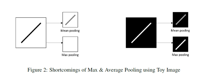
The paper has mentioned some shortcomings for max and average pooling as the most famous simple methods:

Max pooling: takes the maximum value of a region Rij and selecting it for the condensed feature map. It can erase the details of the image (happens if the main details have less intensity than the insignificant details) and also commonly over-fits training data. The equation is:

\begin{align} a_{kij} = max_{(p,q)\in R_{ij}}(a_{kpq}) \end{align}

Average pooling: calculates the average value of a region and selecting it for the condensed feature map. Depending on the data, can dilute pertinent details from an image (happens for data with values much lower than significant details) The equation is:

\begin{align} a_{kij} = \frac{1}{|R_{ij}|}\sum_{(p,q)\in R_{ij}}{{a_{kpq}}} \end{align}

Where [math]\displaystyle{ a_{kij} }[/math] is the output activation of the kth feature map at (i,j), [math]\displaystyle{ a_{kij} }[/math] is the input activation at (p,q) within Rij , and |Rij | is the size of the pooling region.

How the researchers try to combat these issues? Using probabilistic pooling methods such as:

1. Mixed pooling: as a probabilistic pooling method: it combines max and average pooling by randomly selecting one over the other during training in three separate ways:

• For all features within a layer
• Mixed between features within a layer
• Mixed between regions for different features within a layer

The equation is:

\begin{align} a_{kij} = \lambda. max_{(p,q)\in R_{ij}}(a_{kpq})+(1-\lambda).\frac{1}{|R_{ij}|}\sum_{(p,q)\in R_{ij}}{{a_{kpq}}} \end{align}

1. Stochastic pooling: improves upon max pooling by randomly sampling from neighborhood regions based on the probability values of each activation.

\begin{align} a_{kij} = a_l; where: l\sim P(p_1,p_2,...,p_{|R_{ij}|}) \end{align}

This is well described in the figure below:

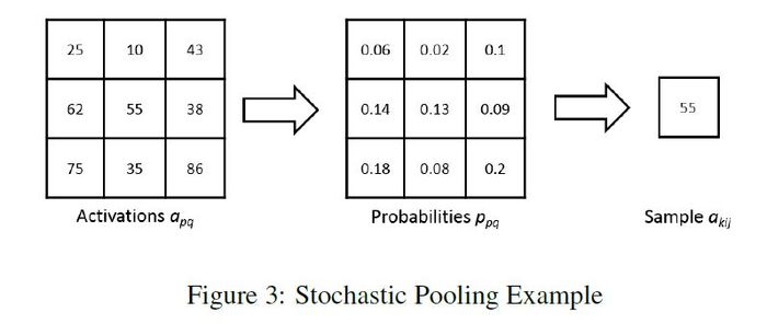
By being based off probability, and not deterministic, stochastic pooling avoids the shortcomings of max and average pooling, while enjoying some of the advantages of max pooling.

Proposed Method

The proposed pooling method uses wavelets to reduce the dimensions of the feature maps. They use wavelet transform to minimize artifacts resulting from neighborhood reduction. They postulate that their approach, which discards the first-order sub-bands, more organically captures the data compression.

• Forward Propagation

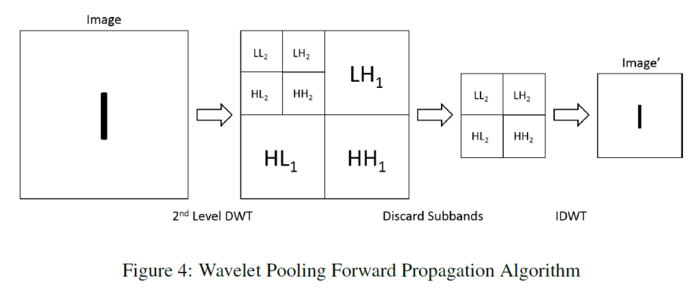
The proposed wavelet pooling scheme pools features by performing a 2nd order decomposition in the wavelet domain according to the fast wavelet transform (FWT) which is a more efficient implementation of the two-dimensional discrete wavelet transform (DWT) as follows:

\begin{align} W_{\varphi}[j+1,k] = h_{\varphi}[-n]*W_{\varphi}[j,n]|_{n=2k,k\leq0} \end{align}

\begin{align} W_{\psi}[j+1,k] = h_{\psi}[-n]*W_{\psi}[j,n]|_{n=2k,k\leq0} \end{align}

where [math]\displaystyle{ \varphi }[/math] is the approximation function, and [math]\displaystyle{ \psi }[/math] is the detail function, [math]\displaystyle{ W_{\varphi},W_{\psi} }[/math] are called approximation and detail coefficients. [math]\displaystyle{ h_{\varphi[-n]} }[/math] and [math]\displaystyle{ h_{\psi[-n]} }[/math] are the time reversed scaling and wavelet vectors, (n) represents the sample in the vector, while (j) denotes the resolution level

When using the FWT on images, it is applied twice (once on the rows, then again on the columns). By doing this in combination, the detail sub-bands (LH, HL, HH) at each decomposition level, and approximation sub-band (LL) for the highest decomposition level is obtained. After performing the 2nd order decomposition, the image features are reconstructed, but only using the 2nd order wavelet sub-bands. This method pools the image features by a factor of 2 using the inverse FWT (IFWT) which is based off the inverse DWT (IDWT).

\begin{align} W_{\varphi}[j,k] = h_{\varphi}[-n]*W_{\varphi}[j+1,n]+h_{\psi}[-n]*W_{\psi}[j+1,n]|_{n=\frac{k}{2},k\leq0} \end{align}

• Backpropagation

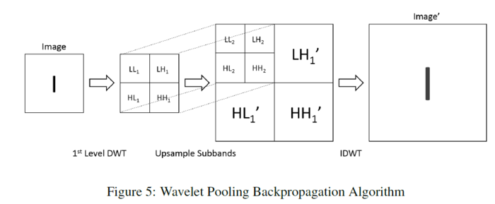
The proposed wavelet pooling algorithm performs backpropagation by reversing the process of its forward propagation. First, the image feature being backpropagated undergoes 1st order wavelet decomposition. After decomposition, the detail coefficient sub-bands up-sample by a factor of 2 to create a new 1st level decomposition. The initial decomposition then becomes the 2nd level decomposition. Finally, this new 2nd order wavelet decomposition reconstructs the image feature for further backpropagation using the IDWT.

Results and discussion

All of their CNN experiments use MatConvNet and stochastic gradient descent is used for training. For the proposed method, the wavelet basis is the Haar wavelet, mainly for its even, square sub-bands They have tested their method on four different datasets as shown in the picture:

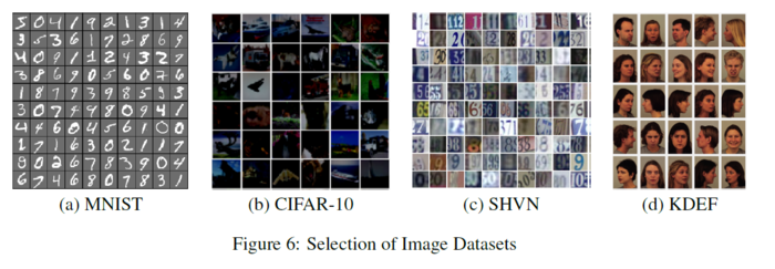
Different methods containing Max, Avg, Mix, Prob, Wavelet have been used and compared with each other at the pooling section of each architecture that is used for different data-sets. The criteria to evaluate the method efficiency are Accuracy and Model Energy.

• MNIST:

The network architecture is based on the example MNIST structure from MatConvNet, with batch-normalization, inserted. All other parameters are the same. The figure below shows their network structure for the MNIST experiments.

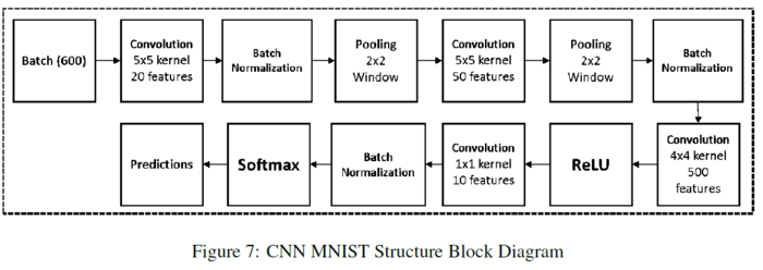
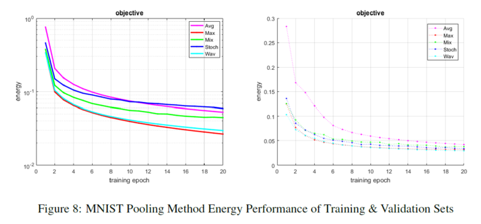
The input training data and test data come from the MNIST database of handwritten digits. The full training set of 60,000 images is used, as well as the full testing set of 10,000 images. The table below shows their proposed method outperforms all methods. Given the small number of epochs, max pooling is the only method to start to over-fit the data during training. Mixed and stochastic pooling show a rocky trajectory but do not over-fit. Average and wavelet pooling show a smoother descent in learning and error reduction. The figure below shows the energy of each method per epoch.

Here is the accuracy for both paradigms:

• CIFAR:

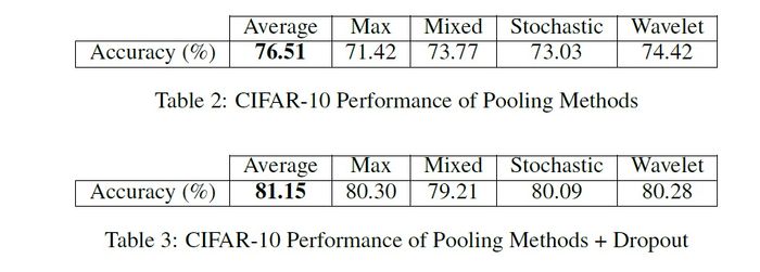
They run two sets of experiments with the pooling methods. The first is a regular network structure with no dropout layers. They use this network to observe each pooling method without extra regularization. The second uses dropout and batch normalization and performs over 30 more epochs to observe the effects of these changes.

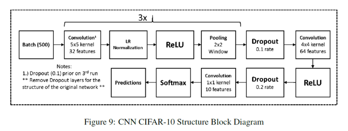
The input training and test data come from the CIFAR-10 dataset. The full training set of 50,000 images is used, as well as the full testing set of 10,000 images. For both cases, with no dropout, and with dropout, Tables below show the proposed method has the second highest accuracy.

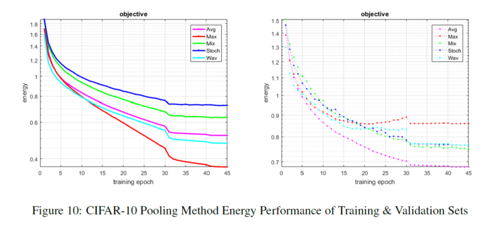
Max pooling over-fits fairly quickly, while wavelet pooling resists over-fitting. The change in learning rate prevents their method from over-fitting, and it continues to show a slower propensity for learning. Mixed and stochastic pooling maintain a consistent progression of learning, and their validation sets trend at a similar, but better rate than their proposed method. Average pooling shows the smoothest descent in learning and error reduction, especially in the validation set. The energy of each method per epoch is also shown below:

• SHVN:

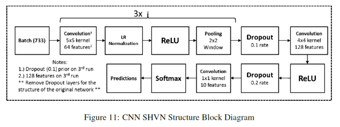
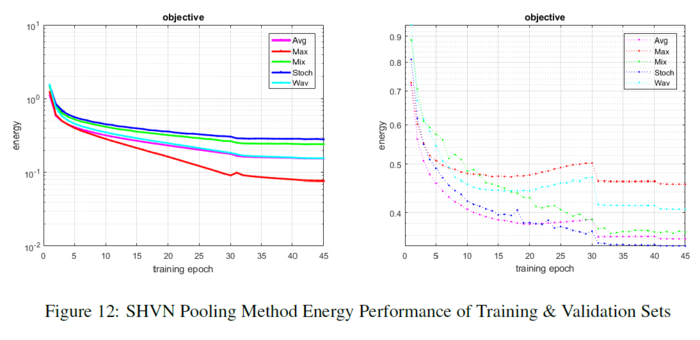
They run two sets of experiments with the pooling methods. The first is a regular network structure with no dropout layers. They use this network to observe each pooling method without extra regularization same as what happened in the previous datasets. The second network uses dropout to observe the effects of this change. The figure below shows their network structure for the SHVN experiments:

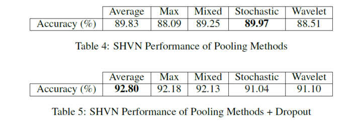
The input training and test data come from the SHVN dataset. For the case with no dropout, they use 55,000 images from the training set. For the case with dropout, they use the full training set of 73,257 images, a validation set of 30,000 images they extract from the extra training set of 531,131 images, as well as the full testing set of 26,032 images. For both cases, with no dropout, and with dropout, Tables below show their proposed method has the second lowest accuracy.

Max and wavelet pooling both slightly over-fit the data. Their method follows the path of max pooling but performs slightly better in maintaining some stability. Mixed, stochastic, and average pooling maintain a slow progression of learning, and their validation sets trend at near identical rates. The figure below shows the energy of each method per epoch.

• KDEF:

They run one set of experiments with the pooling methods that includes dropout. The figure below shows their network structure for the KDEF experiments:

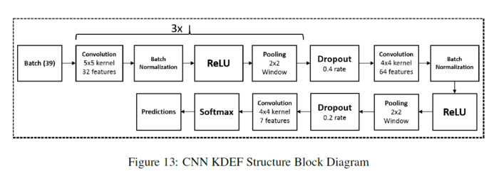
The input training and test data come from the KDEF dataset. This dataset contains 4,900 images of 35 people displaying seven basic emotions (afraid, angry, disgusted, happy, neutral, sad, and surprised) using facial expressions. They display emotions at five poses (full left and right profiles, half left and right profiles, and straight).

This dataset contains a few errors that they have fixed (missing or corrupted images, uncropped images, etc.). All of the missing images are at angles of -90, -45, 45, or 90 degrees. They fix the missing and corrupt images by mirroring their counterparts in MATLAB and adding them back to the dataset. They manually crop the images that need to match the dimensions set by the creators (762 x 562). KDEF does not designate a training or test data set. They shuffle the data and separate 3,900 images as training data, and 1,000 images as test data. They resize the images to 128x128 because of memory and time constraints.

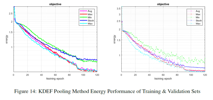
The dropout layers regulate the network and maintain stability in spite of some pooling methods known to over-fit. The table below shows their proposed method has the second highest accuracy. Max pooling eventually over-fits, while wavelet pooling resists over-fitting. Average and mixed pooling resist over-fitting but are unstable for most of the learning. Stochastic pooling maintains a consistent progression of learning. Wavelet pooling also follows a smoother, consistent progression of learning. The figure below shows the energy of each method per epoch.

Here are the accuracy for both paradigms:

Conclusion

They prove wavelet pooling has the potential to equal or eclipse some of the traditional methods currently utilized in CNNs. Their proposed method outperforms all others in the MNIST dataset, outperforms all but one in the CIFAR-10 and KDEF datasets, and performs within respectable ranges of the pooling methods that outdo it in the SHVN dataset. The addition of dropout and batch normalization show their proposed methods response to network regularization. Like the non-dropout cases, it outperforms all but one in both the CIFAR-10 & KDEF datasets and performs within respectable ranges of the pooling methods that outdo it in the SHVN dataset.

Critiques and Suggestions

• The functionality of backpropagation process which can be a positive point of the study is not described enough comparing to the existing methods.
• The main study is on wavelet decomposition while the reason of using Haar as mother wavelet and the number of decomposition levels selection has not been described and are just mentioned as a future study!
• At the beginning, the study mentions that the pooling method is not under attention as it should be. In the end, results show that choosing the pooling method depends on the dataset and they mention trial and test as a reasonable approach to choose the pooling method. In my point of view, the authors have not really been focused on providing a pooling method which can help the current conditions to be improved effectively. At least, trying to extract a better pattern for relating results to the dataset structure could be so helpful.
• Average pooling origins which are mentioned as the main pooling algorithm to compare with, is not even referenced in the introduction.
• Combination of the wavelet, Max and Average pooling can be an interesting option to investigate more on this topic; both in a row(Max/Avg after wavelet pooling) and combined like mix pooling option.

References

Williams, Travis, and Robert Li. "Wavelet Pooling for Convolutional Neural Networks." (2018).