Dynamic Routing Between Capsules STAT946

Presented by

Yang, Tong(Richard)

Hinton's Critiques on CNN

Four arguments against pooling

• It is a bad fit to the psychology of shape perception: It does not explain why we assign intrinsic coordinate frames to objects and why they have such huge effects.

• It solves the wrong problem: We want equivariance, not invariance. Disentangling rather than discarding.

• It fails to use the underlying linear structure: It does not make use of the natural linear manifold that perfectly handles the largest source of variance in images.

• Pooling is a poor way to do dynamic routing: We need to route each part of the input to the neurons that know how to deal with it. Finding the best routing is equivalent to parsing the image.

Equivariance

• Without the sub-sampling, convolutional neural nets give "place-coded" equivariance for discrete translations.

Two types of equivariance

Place-coded equivariance

If a low-level part moves to a very different position it will be represented by a different capsule.

Rate-coded equivariance

If a part only moves a small distance it will be represented by the same capsule but the pose outputs of the capsule will change.

Higher-level capsules have bigger domains so low-level place-coded equivariance gets converted into high-level rate-coded equivariance.

== Extrapolating shape recognition to very different viewpoints

• Current neural net wisdom:
  • Learn different models for different viewpoints.
  • This requires a lot of training data.
• A much better approach:
  • The manifold of images of the same rigid shape is highly non-linear in the space of pixel intensities.
  • Transform to a space in which the manifold is globally linear

Dynamic Routing

In the second section of this paper, authors give a mathematical representations for two key features in routing algorithm in capsule network, which are squashing and agreement. The general setting for this algorithm is between two arbitrary capsules i and j. Capsule j is assumed to be an arbitrary capsule from the first layer of capsules, and capsule i is an arbitrary capsule from the layer below. The purpose of routing algorithm is generate a vector output for routing decision between capsule j and capsule i. Furthermore, this vector output will be used in the decision for choice of dynamic routing.

Routing Algorithm

The routing algorithm is as the following:

Source: Sabour, Frosst, Hinton, 2017

In the following sections, each part of this algorithm will be explained in details.

Log Prior Probability

[math]\displaystyle{ b_{ij} }[/math] represents the log prior probabilities that capsule i should be coupled to capsule j, and updated in each routing iteration. As line 2 suggests, the initial values of [math]\displaystyle{ b_{ij} }[/math] for all possible pairs of capsules are set to 0. In the very first routing iteration, [math]\displaystyle{ b_{ij} }[/math] equals to zero. For each routing iteration, [math]\displaystyle{ b_{ij} }[/math] gets updated by the value of agreement, which will be explained later.

Coupling Coefficient

[math]\displaystyle{ c_{ij} }[/math] represents the coupling coefficient between capsule j and capsule i. It is calculated by applying the softmax function on the log prior probability [math]\displaystyle{ b_{ij} }[/math]. The mathematical transformation is shown below (Equation 3 in paper):

\begin{align} c_{ij} = \frac{exp(b_ij)}{\sum_{k}exp(b_ik)} \end{align}

[math]\displaystyle{ c_{ij} }[/math] are served as weights for computing the weighted sum and probabilities. Therefore, as probabilities, they have the following properties:

\begin{align} c_{ij} \geq 0, \forall i, j \end{align}

and,

\begin{align} \sum_{i,j}c_{ij} = 1, \forall i, j \end{align}

Predicted Output from Layer Below

[math]\displaystyle{ u_{i} }[/math] are the output vector from capsule i in the lower layer, and [math]\displaystyle{ \hat{u}_{j|i} }[/math] are the input vector for capsule j, which are the "prediction vectors" from the capsules in the layer below. [math]\displaystyle{ \hat{u}_{j|i} }[/math] is produced by multiplying [math]\displaystyle{ u_{i} }[/math] by a weight matrix [math]\displaystyle{ W_{ij} }[/math], such as the following:

\begin{align} \hat{u}_{j|i} = W_{ij}u_i \end{align}

where [math]\displaystyle{ W_{ij} }[/math] encodes some spatial relationship between capsule j and capsule i.

Capsule

By using the definitions from previous sections, the total input vector for an arbitrary capsule j can be defined as:

\begin{align} s_j = \sum_{i}c_{ij}\hat{u}_{j|i} \end{align}

which is a weighted sum over all prediction vectors by using coupling coefficients.

Squashing

The length of [math]\displaystyle{ s_j }[/math] is arbitrary, which is needed to be addressed with. The next step is to convert its length between 0 and 1, since we want the length of the output vector of a capsule to represent the probability that the entity represented by the capsule is present in the current input. The "squashing" process is shown below:

\begin{align} v_j = \frac{||s_j||^2}{1+||s_j||^2}\frac{s_j}{||s_j||} \end{align}

Notice that "squashing" is not just normalizing the vector into unit length. In addition, it does extra non-linear transformation to ensure that short vectors get shrunk to almost zero length and long vectors get shrunk to a length slightly below 1. The reason for doing this is to make decision of routing, which is called "routing by agreement" much easier to make between capsule layers.

Agreement

The final step of a routing iteration is to form an routing agreement [math]\displaystyle{ a_{ij} }[/math], which is represents as a scalar product:

\begin{align} a_{ij} = v_{j}\hat{u}_{j|i} \end{align}

As we mentioned in "squashing" section, the length of [math]\displaystyle{ v_{j} }[/math] is either close to 0 or close to 1, which will effect the magnitude of [math]\displaystyle{ a_{ij} }[/math] in this case. Therefore, the magnitude of [math]\displaystyle{ a_{ij} }[/math] indicate the how strong the routing algorithm agrees on taking the route between capsule j and capsule i. For each routing iteration, the log prior probability, [math]\displaystyle{ b_{ij} }[/math] will be updated by adding the value of its agreement value, which will effect how the coupling coefficients are computed in the next routing iteration. Because of the "squashing" process, we will eventually end up with a capsule j with its [math]\displaystyle{ v_{j} }[/math] close to 1 while all other capsules with its [math]\displaystyle{ v_{j} }[/math] close to 0, which indicates that this capsule j should be activated.

CapsNet Architecture

The second part of this paper discuss the experiment results from a 3-layer CapsNet, the architecture can be divided into two parts, encoder and decoder.

Encoder

Source: Sabour, Frosst, Hinton, 2017

How many routing iteration to use?

In appendix A of this paper, the authors have shown the empirical results from 500 epochs of training at different choice of routing iterations. According to their observation, more routing iterations increases the capacity of CapsNet but tends to bring additional risk of overfitting. Moreover, CapsNet with routing iterations less than three are not effective in general. As result, they suggest 3 iterations of routing for all experiments.

Marginal loss for digit existence

The experiments performed include segmenting overlapping digits on MultiMINST data set, so the loss function has be adjusted for presents of multiple digits. The marginal lose [math]\displaystyle{ L_k }[/math] for each capsule k is calculate by:

\begin{align} L_k = T_k max(0, m^+ - ||v_k||)^2 + \lambda(1 - T_k) max(0, ||v_k|| - m^-)^2 \end{align}

where [math]\displaystyle{ m^+ = 0.9 }[/math], [math]\displaystyle{ m^- = 0.1 }[/math], and [math]\displaystyle{ \lambda = 0.5 }[/math].

[math]\displaystyle{ T_k }[/math] is an indicator for presence of digit of class k, it takes value of 1 if and only if class k is presented. If class k is not presented, [math]\displaystyle{ \lambda }[/math] down-weight the loss which shrinks the lengths of the activity vectors for all the digit capsules. By doing this, The loss function penalizes the initial learning for all absent digit class, since we would like the top-level capsule for digit class k to have long instantiation vector if and only if that digit class is present in the input.

Layer 1: Conv1

The first layer of CapsNet. Similar to CNN, this is just convolutional layer that converts pixel intensities to activities of local feature detectors.

• Layer Type: Convolutional Layer.
• Input: [math]\displaystyle{ 28 \times 28 }[/math] pixels.
• Kernel size: [math]\displaystyle{ 9 \times 9 }[/math].
• Number of Kernels: 256.
• Activation function: ReLU.
• Output: [math]\displaystyle{ 20 \times 20 \times 256 }[/math] tensor.

Layer 2: PrimaryCapsules

The second layer is formed by 32 primary 8D capsules. By 8D, it means that each primary capsule contains 8 convolutional units with a [math]\displaystyle{ 9 \times 9 }[/math] kernel and a stride of 2. Each capsule will take a [math]\displaystyle{ 20 \times 20 \times 256 }[/math] tensor from Conv1 and produce an output of a [math]\displaystyle{ 6 \times 6 \times 8 }[/math] tensor.

• Layer Type: Convolutional Layer
• Input: [math]\displaystyle{ 20 \times 20 \times 256 }[/math] tensor.
• Number of capsules: 32.
• Number of convolutional units in each capsule: 8.
• Size of each convolutional unit: [math]\displaystyle{ 6 \times 6 }[/math].
• Output: [math]\displaystyle{ 6 \times 6 \times 8 }[/math] 8-dimensional vectors.

Layer 3: DigitsCaps

The last layer has 10 16D capsules, one for each digit. Not like the PrimaryCapsules layer, this layer is fully connected. Since this is the top capsule layer, dynamic routing mechanism will be applied between DigitsCaps and PrimaryCapsules. The process begins by taking a transformation of predicted output from PrimaryCapsules layer. Each output is a 8-dimensional vector, which needed to be mapped to a 16-dimensional space. Therefore, the weight matrix, [math]\displaystyle{ W_{ij} }[/math] is a [math]\displaystyle{ 8 \times 16 }[/math] matrix. The next step is to acquire coupling coefficients from routing algorithm and to perform "squashing" to get the output.

• Layer Type: Fully connected layer.
• Input: [math]\displaystyle{ 6 \times 6 \times 8 }[/math] 8-dimensional vectors.
• Output: [math]\displaystyle{ 16 \times 10 }[/math] matrix.

The loss function

The output of the loss function would be a ten-dimensional one-hot encoded vector with 9 zeros and 1 one at the correct position.

Regularization Method: Reconstruction

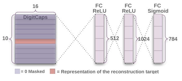
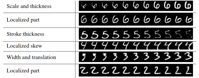
This is regularization method introduced in the implementation of CapsNet. The method is to introduce a reconstruction loss (scaled down by 0.0005) to margin loss during training. The authors argue this would encourage the digit capsules to encode the instantiation parameters the input digits. All the reconstruction during training is by using the true labels of the image input.

Decoder

The decoder consists of 3 fully connected layers, each layer maps pixel intensities to pixel intensities. The number of parameters in each layer and the activation functions used are indicated in the figure below:

Source: Sabour, Frosst, Hinton, 2017

Result

The authors includes some results for CapsNet classification test accuracy to justify the result of reconstruction. We can see that for CapsNet with 1 routing iteration and CapsNet with 3 routing iterations, implement reconstruction shows significant improvements in both MINIST and MultiMINST data set. These improvements show the importance of routing and reconstruction regularizer.

Source: Sabour, Frosst, Hinton, 2017

Experiment Results for CapsNet

MINST

Interpretation of Each Capsule

Source: Sabour, Frosst, Hinton, 2017