On The Convergence Of ADAM And Beyond: Difference between revisions
| Line 1: | Line 1: | ||
= Introduction = | = Introduction = | ||
This paper focuses strictly on the pitfalls in convergence of the ADAM optimizer from a theoretical standpoint and proposes a novel improvement to ADAM called AMSGrad. The paper introduces the idea that it is possible for ADAM to get "stuck" in its weighted average history, preventing it from converging to an optimal solution. For example, in an experiment there may be a large spike in the gradient during some minibatches, but since ADAM weighs the current update by the exponential moving averages of squared past | |||
gradients, the effect of the large spike in gradient is lost. This can be prevented through novel adjustments to the ADAM optimization algorithm, which can improve convergence. | gradients, the effect of the large spike in gradient is lost. This can be prevented through novel but simple adjustments to the ADAM optimization algorithm, which can improve convergence. | ||
== Notation == | == Notation == | ||
The paper presents the following framework | The paper presents the following framework as a generalization to all training algorithms, allowing us to fully define any specific variant such as AMSGrad or SGD entirely within it: | ||
[[File:training_algo_framework.png|700px|center]] | [[File:training_algo_framework.png|700px|center]] | ||
| Line 12: | Line 12: | ||
=== SGD As An Example === | === SGD As An Example === | ||
To recover SGD using this framework we simply select <math> \phi_t (g_1, \dotsc, g_t) = g_t</math>, <math> \psi_t (g_1, \dotsc, g_t) = I </math> and <math>\alpha_t = \alpha / \sqrt{t}</math>. It | To recover SGD using this framework we simply select <math> \phi_t (g_1, \dotsc, g_t) = g_t</math>, <math> \psi_t (g_1, \dotsc, g_t) = I </math> and <math>\alpha_t = \alpha / \sqrt{t}</math>. It is easy to see that no transformations are ultimately applied to any of the parameters based on any gradient history other than the most recent from <math> \phi_t </math> and that <math> \psi_t </math> in no way transforms any of the parameters by any specific amount as <math> V_t = I </math> has no impact later on. | ||
=== ADAGRAD As Another Example === | === ADAGRAD As Another Example === | ||
| Line 19: | Line 19: | ||
=== ADAM As Another Example === | === ADAM As Another Example === | ||
Once you can convince yourself that SGD is correct, you should understand the framework enough to see why the following setup for ADAM will allow us to recover the behaviour we want. ADAM has the ability to define a "learning rate" for every parameter based on how much that parameter moves over time (a.k.a | Once you can convince yourself that the recovery of SGD from the generalized framework is correct, you should understand the framework enough to see why the following setup for ADAM will allow us to recover the behaviour we want. ADAM has the ability to define a "learning rate" for every parameter based on how much that parameter moves over time (a.k.a its momentum) supposedly to help with the learning process. | ||
In order to do this we will choose <math> \phi_t (g_1, \dotsc, g_t) = (1 - \beta_1) \sum_{i=0}^{t} {\beta_1}^{t - i} g_t </math>, psi to be <math> \psi_t (g_1, \dotsc, g_t) = (1 - \beta_2)</math>diag<math>( \sum_{i=0}^{t} {\beta_2}^{t - i} {g_t}^2) </math>, and keep <math>\alpha_t = \alpha / \sqrt{t}</math>. This | In order to do this, we will choose <math> \phi_t (g_1, \dotsc, g_t) = (1 - \beta_1) \sum_{i=0}^{t} {\beta_1}^{t - i} g_t </math>, psi to be <math> \psi_t (g_1, \dotsc, g_t) = (1 - \beta_2)</math>diag<math>( \sum_{i=0}^{t} {\beta_2}^{t - i} {g_t}^2) </math>, and keep <math>\alpha_t = \alpha / \sqrt{t}</math>. This setup is equivalent to choosing a learning rate decay of <math>\alpha / \sqrt{\sum_i g_{i,j}}</math> for <math>j \in [d]</math>. | ||
From this, we can now see that <math>m_t </math> gets filled up with the exponentially weighted average of the history of our gradients that we | From this, we can now see that <math>m_t </math> gets filled up with the exponentially weighted average of the history of our gradients that we have come across so far in the algorithm. And that as we proceed to update we scale each one of our parameters by dividing out <math> V_t </math> (in the case of diagonal it is just one over the diagonal entry) which contains the exponentially weighted average of each parameter's momentum (<math> {g_t}^2 </math>) across our training so far in the algorithm. Thus each parameter has its own unique scaling by its second moment or momentum. Intuitively, from a physical perspective, if each parameter is a ball rolling around in the optimization landscape what we are now doing is instead of having the ball change positions on the landscape at a fixed velocity (i.e. momentum of 0) the ball now has the ability to accelerate and speed up or slow down if it is on a steep hill or flat trough in the landscape (i.e. a momentum that can change with time). | ||
= <math> \Gamma_t </math>, an Interesting Quantity = | = <math> \Gamma_t </math>, an Interesting Quantity = | ||
Revision as of 22:15, 2 April 2018
Introduction
This paper focuses strictly on the pitfalls in convergence of the ADAM optimizer from a theoretical standpoint and proposes a novel improvement to ADAM called AMSGrad. The paper introduces the idea that it is possible for ADAM to get "stuck" in its weighted average history, preventing it from converging to an optimal solution. For example, in an experiment there may be a large spike in the gradient during some minibatches, but since ADAM weighs the current update by the exponential moving averages of squared past gradients, the effect of the large spike in gradient is lost. This can be prevented through novel but simple adjustments to the ADAM optimization algorithm, which can improve convergence.
Notation
The paper presents the following framework as a generalization to all training algorithms, allowing us to fully define any specific variant such as AMSGrad or SGD entirely within it:

Where we have [math]\displaystyle{ x_t }[/math] as our network parameters defined within a vector space [math]\displaystyle{ \mathcal{F} }[/math]. [math]\displaystyle{ \prod_{\mathcal{F}} (y) = }[/math] the projection of [math]\displaystyle{ y }[/math] on to the set [math]\displaystyle{ \mathcal{F} }[/math]. [math]\displaystyle{ \psi_t }[/math] and [math]\displaystyle{ \phi_t }[/math] correspond to arbitrary functions we will provide later, The former maps from the history of gradients to [math]\displaystyle{ \mathbb{R}^d }[/math] and the latter maps from the history of the gradients to positive semi definite matrices. And finally [math]\displaystyle{ f_t }[/math] is our loss function at some time [math]\displaystyle{ t }[/math], the rest should be pretty self explanatory. Using this framework and defining different [math]\displaystyle{ \psi_t }[/math] , [math]\displaystyle{ \phi_t }[/math] will allow us to recover all different kinds of training algorithms under this one roof.
SGD As An Example
To recover SGD using this framework we simply select [math]\displaystyle{ \phi_t (g_1, \dotsc, g_t) = g_t }[/math], [math]\displaystyle{ \psi_t (g_1, \dotsc, g_t) = I }[/math] and [math]\displaystyle{ \alpha_t = \alpha / \sqrt{t} }[/math]. It is easy to see that no transformations are ultimately applied to any of the parameters based on any gradient history other than the most recent from [math]\displaystyle{ \phi_t }[/math] and that [math]\displaystyle{ \psi_t }[/math] in no way transforms any of the parameters by any specific amount as [math]\displaystyle{ V_t = I }[/math] has no impact later on.
ADAGRAD As Another Example
To recover ADAGRAD, we select [math]\displaystyle{ \phi_t (g_1, \dotsc, g_t) = g_t }[/math], [math]\displaystyle{ \psi_t (g_1, \dotsc, g_t) = \frac{\sum_{i=1}^{t} g_i^2}{t} }[/math], and [math]\displaystyle{ \alpha_t = \alpha / \sqrt{t} }[/math]. Therefore, compared to SGD, ADAGRAD uses a different step size for each parameter, based on the past gradients for that parameter; the learning rate becomes [math]\displaystyle{ \alpha_t = \alpha / \sqrt{\sum_i g_{i,j}^2} }[/math] for each parameter [math]\displaystyle{ j }[/math]. The authors note that this scheme is quite efficient when the gradients are sparse.
ADAM As Another Example
Once you can convince yourself that the recovery of SGD from the generalized framework is correct, you should understand the framework enough to see why the following setup for ADAM will allow us to recover the behaviour we want. ADAM has the ability to define a "learning rate" for every parameter based on how much that parameter moves over time (a.k.a its momentum) supposedly to help with the learning process.
In order to do this, we will choose [math]\displaystyle{ \phi_t (g_1, \dotsc, g_t) = (1 - \beta_1) \sum_{i=0}^{t} {\beta_1}^{t - i} g_t }[/math], psi to be [math]\displaystyle{ \psi_t (g_1, \dotsc, g_t) = (1 - \beta_2) }[/math]diag[math]\displaystyle{ ( \sum_{i=0}^{t} {\beta_2}^{t - i} {g_t}^2) }[/math], and keep [math]\displaystyle{ \alpha_t = \alpha / \sqrt{t} }[/math]. This setup is equivalent to choosing a learning rate decay of [math]\displaystyle{ \alpha / \sqrt{\sum_i g_{i,j}} }[/math] for [math]\displaystyle{ j \in [d] }[/math].
From this, we can now see that [math]\displaystyle{ m_t }[/math] gets filled up with the exponentially weighted average of the history of our gradients that we have come across so far in the algorithm. And that as we proceed to update we scale each one of our parameters by dividing out [math]\displaystyle{ V_t }[/math] (in the case of diagonal it is just one over the diagonal entry) which contains the exponentially weighted average of each parameter's momentum ([math]\displaystyle{ {g_t}^2 }[/math]) across our training so far in the algorithm. Thus each parameter has its own unique scaling by its second moment or momentum. Intuitively, from a physical perspective, if each parameter is a ball rolling around in the optimization landscape what we are now doing is instead of having the ball change positions on the landscape at a fixed velocity (i.e. momentum of 0) the ball now has the ability to accelerate and speed up or slow down if it is on a steep hill or flat trough in the landscape (i.e. a momentum that can change with time).
[math]\displaystyle{ \Gamma_t }[/math], an Interesting Quantity
Now that we have an idea of what ADAM looks like in this framework, let us now investigate the following:
Which essentially measure the change of the "Inverse of the learning rate" across time (since we are using alpha's as step sizes). A key observation is that for SGD and ADAGRAD, [math]\displaystyle{ \Gamma_t \succeq 0 }[/math] for all [math]\displaystyle{ t \in [T] }[/math], which simply follows from the update rules of SGD and ADAGRAD. Looking back to our example of SGD it's not hard to see that this quantity is strictly positive semidefinite, which leads to "non-increasing" learning rates, which is a desired property. However, that is not the case with ADAM, and can pose a problem in a theoretical and applied setting. The problem ADAM can face is that [math]\displaystyle{ \Gamma_t }[/math] can potentially be indefinite for [math]\displaystyle{ t \in [T] }[/math], which the original proof assumed it could not be. The math for this proof is VERY long so instead we will opt for an example to showcase why this could be an issue.
Consider the loss function [math]\displaystyle{ f_t(x) = \begin{cases} Cx & \text{for } t \text{ mod 3} = 1 \\ -x & \text{otherwise} \end{cases} }[/math]
Where we have [math]\displaystyle{ C \gt 2 }[/math] and [math]\displaystyle{ \mathcal{F} }[/math] is [math]\displaystyle{ [-1,1] }[/math]. Additionally we choose [math]\displaystyle{ \beta_1 = 0 }[/math] and [math]\displaystyle{ \beta_2 = 1/(1+C^2) }[/math]. We then proceed to plug this into our framework from before. This function is periodic and it's easy to see that it has the gradient of C once and then a gradient of -1 twice every period. It has an optimal solution of [math]\displaystyle{ x = -1 }[/math] (from a regret standpoint), but using ADAM we would eventually converge at [math]\displaystyle{ x = 1 }[/math], since [math]\displaystyle{ \psi_t }[/math] would scale down the [math]\displaystyle{ C }[/math] by a factor of almost [math]\displaystyle{ C }[/math] so that it's unable to "overpower" the multiple -1's.
We formalize this intuition in the results below.
Theorem 1. There is an online convex optimization problem where ADAM has non-zero average regret. i.e. [math]\displaystyle{ R_T/T\nrightarrow 0 }[/math] as [math]\displaystyle{ T\rightarrow \infty }[/math].
One might think that adding a small constant in the denominator of the update function can help avoid this issue by modifying the update for ADAM as follow: \begin{align} \hat x_{t+1} = x_t - \alpha_t m_t/\sqrt{V_t + \epsilon \mathbb{I}} \end{align}
The selection of [math]\displaystyle{ \epsilon }[/math] appears to be crucial for the performance of the algorithm in practice. However, this work shows that for any constant [math]\displaystyle{ \epsilon \gt 0 }[/math], there exists an online optimization setting where ADAM has non-zero average regret asymptotically.
Theorem 2. For any constant [math]\displaystyle{ \beta_1,\beta_2 \in [0,1) }[/math] such that [math]\displaystyle{ \beta_2 \lt \sqrt{\beta_2} }[/math], there is an online convex optimization problem where ADAM has non-zero average regret i.e. [math]\displaystyle{ R_T/T\nrightarrow 0 }[/math] as [math]\displaystyle{ T\rightarrow \infty }[/math].
Theorem 3. For any constant [math]\displaystyle{ \beta_1,\beta_2 \in [0,1) }[/math] such that [math]\displaystyle{ \beta_2 \lt \sqrt{\beta_2} }[/math], there is a stochastic convex optimization problem for which ADAM does not converge to the optimal solution.
AMSGrad as an improvement to ADAM
There is a very simple intuitive fix to ADAM to handle this problem. We simply scale our historical weighted average by the maximum we have seen so far to avoid the negative sign problem. There is a very simple one-liner adaptation of ADAM to get to AMSGRAD:

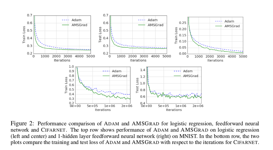
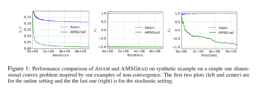
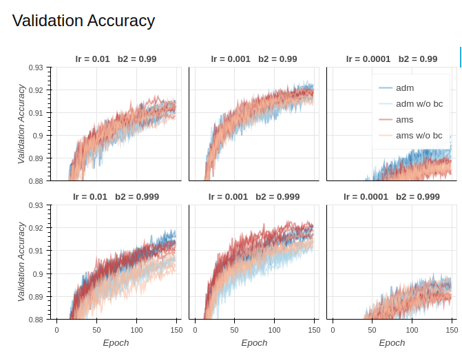
Below are some simple plots comparing ADAM and AMSGrad, the first are from the paper and the second are from another individual who attempted to recreate the experiments. The two plots somewhat disagree with one another so take this heuristic improvement with a grain of salt.

Here is another example of a one-dimensional convex optimization problem where ADAM fails to converge


Conclusion
We have introduced a framework for which we could view several different training algorithms. From there we used it to recover SGD as well as ADAM. In our recovery of ADAM we investigated the change of the inverse of the learning rate over time to discover in certain cases there were convergence issues. We proposed a new heuristic AMSGrad to help deal with this problem and presented some empirical results that show it may have helped ADAM slightly. Thanks for your time.
Critique
The contrived example which serves as the intuition to illustrate the failure of ADAM is not convincing, since we can construct similar failure examples for SGD as well. Consider the loss function
[math]\displaystyle{ f_t(x) = \begin{cases} -x & \text{for } t \text{ mod 2} = 1 \\ -\frac{1}{2} x^2 & \text{otherwise} \end{cases} }[/math]
where [math]\displaystyle{ x \in \mathcal{F} = [-a, 1], a \in [1, \sqrt{2}) }[/math]. The optimal solution is [math]\displaystyle{ x=1 }[/math], but starting from initial point [math]\displaystyle{ x_{t=0} \le -1 }[/math], SGD will converge to [math]\displaystyle{ x = -a }[/math]
Source
1. Sashank J. Reddi and Satyen Kale and Sanjiv Kumar. "On the Convergence of Adam and Beyond." International Conference on Learning Representations. 2018