End-to-End Differentiable Adversarial Imitation Learning

Introduction

The ability to imitate an expert policy is very beneficial in the case of automating human demonstrated tasks. Assuming that a sequence of state action pairs (trajectories) of an expert policy are available, a new policy can be trained that imitates the expert without having access to the original reward signal used by the expert. There are two main approaches to solve the problem of imitating a policy; they are Behavioural Cloning (BC) and Inverse Reinforcement Learning (IRL). BC directly learns the conditional distribution of actions over states in a supervised fashion by training on single time-step state-action pairs. The disadvantage of BC is that the training requires large amounts of expert data, which is hard to obtain. In addition, an agent trained using BC is unaware of how its action can affect future state distribution. The second method using IRL involves recovering a reward signal under which the expert is uniquely optimal; the main disadvantage is that it’s an ill-posed problem.

To address the problem of imitating an expert policy, techniques based on Generative Adversarial Networks (GANs) have been proposed in recent years. GANs use a discriminator to guide the generative model towards producing patterns like those of the expert. This idea was used by (Ho & Ermon, 2016) in their work titled Generative Adversarial Imitation Learning (GAIL) to imitate an expert policy in a model-free setup. A model free setup is the one where the agent cannot make predictions about what the next state and reward will be before it takes each action since the transition function to move from state A to state B is not learned. The disadvantage of GAIL’s model-free approach is that backpropagation required gradient estimation which tends to suffer from high variance, which results in the need for large sample sizes and variance reduction methods. This paper proposed a model-based method (MGAIL) to address these issues by training a policy which is represented by the information propagated from the discriminator to the generator..

Background

Markov Decision Process

Consider an infinite-horizon discounted Markov decision process (MDP), defined by the tuple [math]\displaystyle{ (S, A, P, r, \rho_0, \gamma) }[/math] where [math]\displaystyle{ S }[/math] is the set of states, [math]\displaystyle{ A }[/math] is a set of actions, [math]\displaystyle{ P : S × A × S → [0, 1] }[/math] is the transition probability distribution, [math]\displaystyle{ r : (S × A) → R }[/math] is the reward function, [math]\displaystyle{ \rho_0 : S → [0, 1] }[/math] is the distribution over initial states, and [math]\displaystyle{ γ ∈ (0, 1) }[/math] is the discount factor. Let [math]\displaystyle{ π }[/math] denote a stochastic policy [math]\displaystyle{ π : S × A → [0, 1] }[/math], [math]\displaystyle{ R(π) }[/math] denote its expected discounted reward: [math]\displaystyle{ E_πR = E_π [\sum_{t=0}^T \gamma^t r_t] }[/math] and [math]\displaystyle{ τ }[/math] denote a trajectory of states and actions [math]\displaystyle{ τ = {s_0, a_0, s_1, a_1, ...} }[/math].

Imitation Learning

A common technique for performing imitation learning is to train a policy [math]\displaystyle{ \pi }[/math] that minimizes some loss function [math]\displaystyle{ l(s, \pi(s)) }[/math] with respect to a discounted state distribution encountered by the expert: [math]\displaystyle{ d_\pi(s) = (1-\gamma)\sum_{t=0}^{\infty}\gamma^t p(s_t) }[/math]. This can be obtained using any supervised learning (SL) algorithm, but the policy's prediction affects future state distributions; this violates the independent and identically distributed (i.i.d) assumption made by most SL algorithms. This process is susceptible to compounding errors since a slight deviation in the learner's behavior can lead to different state distributions not encountered by the expert policy.

This issue was overcome through the use of the Forward Training (FT) algorithm which trains a non-stationary policy iteratively over time. At each time step a new policy is trained on the state distribution induced by the previously trained policies [math]\displaystyle{ \pi_0 }[/math], [math]\displaystyle{ \pi_1 }[/math], ...[math]\displaystyle{ \pi_{t-1} }[/math]. This is continued till the end of the time horizon to obtain a policy that can mimic the expert policy. This requirement to train a policy at each time step till the end makes the FT algorithm impractical for cases where the time horizon is very large or undefined. This shortcoming is resolved using the Stochastic Mixing Iterative Learning (SMILe) algorithm. SMILe trains a stochastic stationary policy over several iterations under the trajectory distribution induced by the previously trained policy: [math]\displaystyle{ \pi_t = \pi_{t-1} + \alpha (1 - \alpha)^{t-1}(\hat{\pi}_t - \pi_0) }[/math], with [math]\displaystyle{ \pi_0 }[/math] following expert's policy at the start of training.

Generative Adversarial Networks

GANs learn a generative model that can fool the discriminator by using a two-player zero-sum game:

\begin{align} \underset{G}{\operatorname{argmin}}\; \underset{D\in (0,1)}{\operatorname{argmax}} = \mathbb{E}_{x\sim p_E}[log(D(x)]\ +\ \mathbb{E}_{z\sim p_z}[log(1 - D(G(z)))] \end{align}

In the above equation, [math]\displaystyle{ p_E }[/math] represents the expert distribution and [math]\displaystyle{ p_z }[/math] represents the input noise distribution from which the input to the generator is sampled. The generator produces patterns and the discriminator judges if the pattern was generated or from the expert data. When the discriminator cannot distinguish between the two distributions the game ends and the generator has learned to mimic the expert. GANs rely on basic ideas such as binary classification and algorithms such as backpropagation in order to learn the expert distribution.

GAIL applies GANs to the task of imitating an expert policy in a model-free approach. GAIL uses similar objective functions like GANs, but the expert distribution in GAIL represents the joint distribution over state action tuples:

\begin{align} \underset{\pi}{\operatorname{argmin}}\; \underset{D\in (0,1)}{\operatorname{argmax}} = \mathbb{E}_{\pi}[log(D(s,a)]\ +\ \mathbb{E}_{\pi_E}[log(1 - D(s,a))] - \lambda H(\pi)) \end{align}

where [math]\displaystyle{ H(\pi) \triangleq \mathbb{E}_{\pi}[-log\: \pi(a|s)] }[/math] is the entropy.

This problem cannot be solved using the standard methods described for GANs because the generator in GAIL represents a stochastic policy. The exact form of the first term in the above equation is given by: [math]\displaystyle{ \mathbb{E}_{s\sim \rho_\pi(s)}\mathbb{E}_{a\sim \pi(\cdot |s)} [log(D(s,a)] }[/math].

The two-player game now depends on the stochastic properties ([math]\displaystyle{ \theta }[/math]) of the policy, and it is unclear how to differentiate the above equation with respect to [math]\displaystyle{ \theta }[/math]. This problem can be overcome using score functions such as REINFORCE to obtain an unbiased gradient estimation:

\begin{align} \nabla_\theta\mathbb{E}_{\pi} [log\; D(s,a)] \cong \hat{\mathbb{E}}_{\tau_i}[\nabla_\theta\; log\; \pi_\theta(a|s)Q(s,a)] \end{align}

where [math]\displaystyle{ Q(\hat{s},\hat{a}) }[/math] is the score function of the gradient:

\begin{align} Q(\hat{s},\hat{a}) = \hat{\mathbb{E}}_{\tau_i}[log\; D(s,a) | s_0 = \hat{s}, a_0 = \hat{a}] \end{align}

REINFORCE gradients suffer from high variance which makes them difficult to work with even after applying variance reduction techniques. In order to better understand the changes required to fool the discriminator we need access to the gradients of the discriminator network, which can be obtained from the Jacobian of the discriminator. This paper demonstrates the use of a forward model along with the Jacobian of the discriminator to train a policy, without using high-variance gradient estimations.

Algorithm

This section first analyzes the characteristics of the discriminator network, then describes how a forward model can enable policy imitation through GANs. Lastly, the model based adversarial imitation learning algorithm is presented.

The discriminator network

The discriminator network is trained to predict the conditional distribution: [math]\displaystyle{ D(s,a) = p(y|s,a) }[/math] where [math]\displaystyle{ y \in (\pi_E, \pi) }[/math].

The discriminator is trained on an even distribution of expert and generated examples; hence [math]\displaystyle{ p(\pi) = p(\pi_E) = \frac{1}{2} }[/math]. Given this and applying Bayes' theorem, we can rearrange and factor [math]\displaystyle{ D(s,a) }[/math] to obtain:

\begin{aligned} D(s,a) &= p(\pi|s,a) \\ & = \frac{p(s,a|\pi)p(\pi)}{p(s,a|\pi)p(\pi) + p(s,a|\pi_E)p(\pi_E)} \\ & = \frac{p(s,a|\pi)}{p(s,a|\pi) + p(s,a|\pi_E)} \\ & = \frac{1}{1 + \frac{p(s,a|\pi_E)}{p(s,a|\pi)}} \\ & = \frac{1}{1 + \frac{p(a|s,\pi_E)}{p(a|s,\pi)} \cdot \frac{p(s|\pi_E)}{p(s|\pi)}} \\ \end{aligned}

Define [math]\displaystyle{ \varphi(s,a) }[/math] and [math]\displaystyle{ \psi(s) }[/math] to be:

\begin{aligned} \varphi(s,a) = \frac{p(a|s,\pi_E)}{p(a|s,\pi)}, \psi(s) = \frac{p(s|\pi_E)}{p(s|\pi)} \end{aligned}

to get the final expression for [math]\displaystyle{ D(s,a) }[/math]: \begin{aligned} D(s,a) = \frac{1}{1 + \varphi(s,a)\cdot \psi(s)} \end{aligned}

[math]\displaystyle{ \varphi(s,a) }[/math] represents a policy likelihood ratio, and [math]\displaystyle{ \psi(s) }[/math] represents a state distribution likelihood ratio. Based on these expressions, the paper states that the discriminator makes its decisions by answering two questions. The first question relates to state distribution: what is the likelihood of encountering state [math]\displaystyle{ s }[/math] under the distribution induces by [math]\displaystyle{ \pi_E }[/math] vs [math]\displaystyle{ \pi }[/math]? The second question is about behavior: given a state [math]\displaystyle{ s }[/math], how likely is action a under [math]\displaystyle{ \pi_E }[/math] vs [math]\displaystyle{ \pi }[/math]? The desired change in state is given by [math]\displaystyle{ \psi_s \equiv \partial \psi / \partial s }[/math]; this information can by obtained from the partial derivatives of [math]\displaystyle{ D(s,a) }[/math], which is why these derivatives are proposed to be used for training policies (see following sections):

\begin{aligned} \nabla_aD &= - \frac{\varphi_a(s,a)\psi(s)}{(1 + \varphi(s,a)\psi(s))^2} \\ \nabla_sD &= - \frac{\varphi_s(s,a)\psi(s) + \varphi(s,a)\psi_s(s)}{(1 + \varphi(s,a)\psi(s))^2} \\ \end{aligned}

Backpropagating through stochastic units

There is interest in training stochastic policies because stochasticity encourages exploration for Policy Gradient methods. This is a problem for algorithms that build differentiable computation graphs where the gradients flow from one component to another since it is unclear how to backpropagate through stochastic units. The following subsections show how to estimate the gradients of continuous and categorical stochastic elements for continuous and discrete action domains respectively.

Continuous Action Distributions

In the case of continuous action policies, re-parameterization was used to enable computing the derivatives of stochastic models. Assuming that the stochastic policy has a Gaussian distribution [math]\displaystyle{ \mathcal{N}(\mu_{\theta} (s), \sigma_{\theta}^2 (s)) }[/math], where the mean and variance are given by some deterministic functions [math]\displaystyle{ \mu_{\theta} }[/math] and [math]\displaystyle{ \sigma_{\theta} }[/math], then the policy [math]\displaystyle{ \pi }[/math] can be written as [math]\displaystyle{ \pi_\theta(a|s) = \mu_\theta(s) + \xi \sigma_\theta(s) }[/math], where [math]\displaystyle{ \xi \sim N(0,1) }[/math]. This way, the authors are able to get a Monte-Carlo estimator of the derivative of the expected value of [math]\displaystyle{ D(s, a) }[/math] with respect to [math]\displaystyle{ \theta }[/math]:

\begin{align} \nabla_\theta\mathbb{E}_{\pi(a|s)}D(s,a) = \mathbb{E}_{\rho (\xi )}\nabla_a D(a,s) \nabla_\theta \pi_\theta(a|s) \cong \frac{1}{M}\sum_{i=1}^{M} \nabla_a D(s,a) \nabla_\theta \pi_\theta(a|s)\Bigr|_{\substack{\xi=\xi_i}} \end{align}

Categorical Action Distributions

In the case of discrete action domains, the paper uses categorical re-parameterization with Gumbel-Softmax. This method relies on the Gumbel-Max trick which is a method for drawing samples from a categorical distribution with class probabilities [math]\displaystyle{ \pi(a_1|s),\pi(a_2|s),...,\pi(a_N|s) }[/math]:

\begin{align} a_{argmax} = \underset{i}{argmax}[g_i + log\ \pi(a_i|s)]\textrm{, where } g_i \sim Gumbel(0, 1). \end{align}

Gumbel-Softmax provides a differentiable approximation of the samples obtained using the Gumbel-Max trick:

\begin{align} a_{softmax} = \frac{exp[\frac{1}{\tau}(g_i + log\ \pi(a_i|s))]}{\sum_{j=1}^{k}exp[\frac{1}{\tau}(g_j + log\ \pi(a_i|s))]} \end{align}

In the above equation, the hyper-parameter [math]\displaystyle{ \tau }[/math] (temperature) trades bias for variance. When [math]\displaystyle{ \tau }[/math] gets closer to zero, the softmax operator acts like argmax resulting in a low bias, but high variance; vice versa when the [math]\displaystyle{ \tau }[/math] is large.

The authors use [math]\displaystyle{ a_{softmax} }[/math] to interact with the environment; argmax is applied over [math]\displaystyle{ a_{softmax} }[/math] to obtain a single “pure” action, but the continuous approximation is used in the backward pass using the estimation: [math]\displaystyle{ \nabla_\theta\; a_{argmax} \approx \nabla_\theta\; a_{softmax} }[/math].

Backpropagating through a Forward model

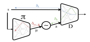
The above subsections presented the means for extracting the partial derivative [math]\displaystyle{ \nabla_aD }[/math]. The main contribution of this paper is incorporating the use of [math]\displaystyle{ \nabla_sD }[/math]. In a model-free approach the state [math]\displaystyle{ s }[/math] is treated as a fixed input, therefore [math]\displaystyle{ \nabla_sD }[/math] is discarded. This is illustrated in Figure 1. This work uses a model-based approach which makes incorporating [math]\displaystyle{ \nabla_sD }[/math] more involved. In the model-based approach, a state [math]\displaystyle{ s_t }[/math] can be written as a function of the previous state action pair: [math]\displaystyle{ s_t = f(s_{t-1}, a_{t-1}) }[/math], where [math]\displaystyle{ f }[/math] represents the forward model. Using the forward model and the law of total derivatives we get:

\begin{align} \nabla_\theta D(s_t,a_t)\Bigr|_{\substack{s=s_t, a=a_t}} &= \frac{\partial D}{\partial a}\frac{\partial a}{\partial \theta}\Bigr|_{\substack{a=a_t}} + \frac{\partial D}{\partial s}\frac{\partial s}{\partial \theta}\Bigr|_{\substack{s=s_t}} \\ &= \frac{\partial D}{\partial a}\frac{\partial a}{\partial \theta}\Bigr|_{\substack{a=a_t}} + \frac{\partial D}{\partial s}\left (\frac{\partial f}{\partial s}\frac{\partial s}{\partial \theta}\Bigr|_{\substack{s=s_{t-1}}} + \frac{\partial f}{\partial a}\frac{\partial a}{\partial \theta}\Bigr|_{\substack{a=a_{t-1}}} \right ) \end{align}

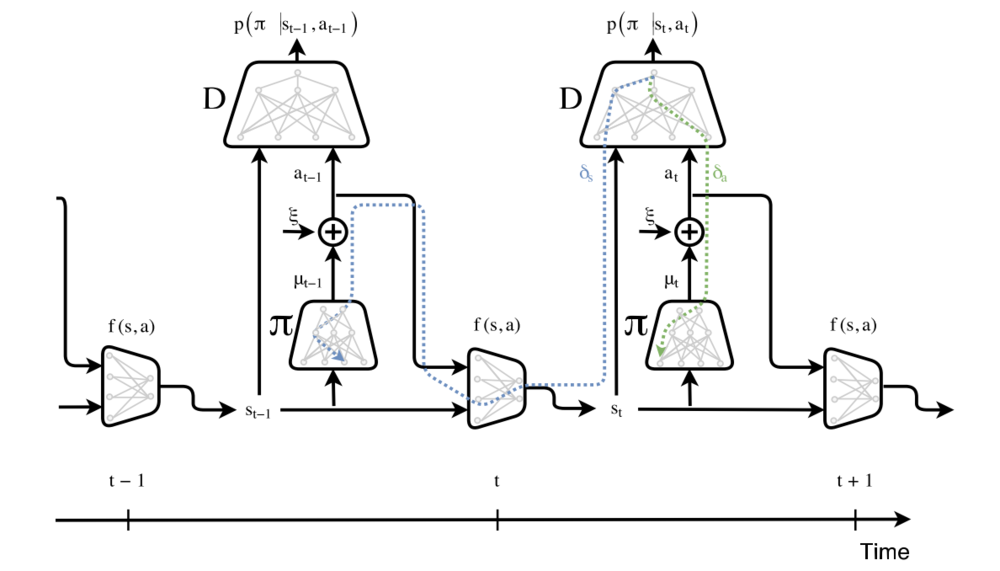
Using this formula, the error regarding deviations of future states [math]\displaystyle{ (\psi_s) }[/math] propagate back in time and influence the actions of policies in earlier times. This is summarized in Figure 2.

Figure 1: Block-diagram of the model-free approach: given a state [math]\displaystyle{ s }[/math], the policy outputs [math]\displaystyle{ \mu }[/math] which is fed to a stochastic sampling unit. An action [math]\displaystyle{ a }[/math] is sampled, and together with [math]\displaystyle{ s }[/math] are presented to the discriminator network. In the backward phase, the error message [math]\displaystyle{ \delta_a }[/math] is blocked at the stochastic sampling unit. From there, a high-variance gradient estimation is used ([math]\displaystyle{ \delta_{HV} }[/math]). Meanwhile, the error message [math]\displaystyle{ \delta_s }[/math] is flushed.

Figure 2: Block diagram of model-based adversarial imitation learning. This diagram describes the computation graph for training the policy (i.e. G). The discriminator network D is fixed at this stage and is trained separately. At time [math]\displaystyle{ t }[/math] of the forward pass, [math]\displaystyle{ \pi }[/math] outputs a distribution over actions: [math]\displaystyle{ \mu_t = \pi(s_t) }[/math], from which an action at is sampled. For example, in the continuous case, this is done using the re-parametrization trick: [math]\displaystyle{ a_t = \mu_t + \xi \cdot \sigma }[/math], where [math]\displaystyle{ \xi \sim N(0,1) }[/math]. The next state [math]\displaystyle{ s_{t+1} = f(s_t, a_t) }[/math] is computed using the forward model (which is also trained separately), and the entire process repeats for time [math]\displaystyle{ t+1 }[/math]. In the backward pass, the gradient of [math]\displaystyle{ \pi }[/math] is comprised of a.) the error message [math]\displaystyle{ \delta_a }[/math] (Green) that propagates fluently through the differentiable approximation of the sampling process. And b.) the error message [math]\displaystyle{ \delta_s }[/math] (Blue) of future time-steps, that propagate back through the differentiable forward model.

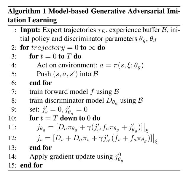
MGAIL Algorithm

Shalev- Shwartz et al. (2016) and Heess et al. (2015) built a multi-step computation graph for describing the familiar policy gradient objective; in this case it is given by:

\begin{align} J(\theta) = \mathbb{E}\left [ \sum_{t=0}^{T} \gamma ^t D(s_t,a_t)|\theta\right ] \end{align}

Using the results from Heess et al. (2015) this paper demonstrates how to differentiate [math]\displaystyle{ J(\theta) }[/math] over a trajectory of [math]\displaystyle{ (s,a,s’) }[/math] transitions:

\begin{align} J_s &= \mathbb{E}_{p(a|s)}\mathbb{E}_{p(s'|s,a)}\left [ D_s + D_a \pi_s + \gamma J'_{s'}(f_s + f_a \pi_s) \right] \\ J_\theta &= \mathbb{E}_{p(a|s)}\mathbb{E}_{p(s'|s,a)}\left [ D_a \pi_\theta + \gamma (J'_{s'} f_a \pi_\theta + J'_\theta) \right] \end{align}

The policy gradient [math]\displaystyle{ \nabla_\theta J }[/math] is calculated by applying equations 12 and 13 recursively for [math]\displaystyle{ T }[/math] iterations. The MGAIL algorithm is presented below.

Forward Model Structure

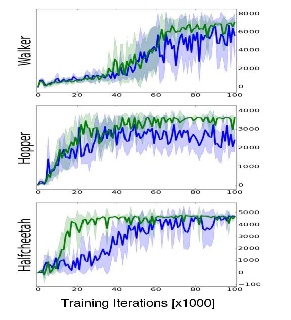
The stability of the learning process depends on the prediction accuracy of the forward model, but learning an accurate forward model is challenging by itself. The authors propose methods for improving the performance of the forward model based on two aspects of its functionality. First, the forward model should learn to use the action as an operator over the state space. To accomplish this, the actions and states, which are sampled form different distributions need to be first represented in a shared space. This is done by encoding the state and action using two separate neural networks and combining their outputs to form a single vector. Additionally, multiple previous states are used to predict the next state by representing the environment as an [math]\displaystyle{ n^{th} }[/math] order MDP. A gated recurrent units (GRU, a simpler variant on the LSTM model) layer is incorporated into the state encoder to enable recurrent connections from previous states. Using these modifications, the model is able to achieve better, and more stable results compared to the standard forward model based on a feed forward neural network. The comparison is presented in Figure 3.

Figure 3: Performance comparison between a basic forward model (Blue), and the advanced forward model (Green).

Experiments

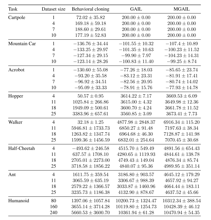
The proposed algorithm is evaluated on three discrete control tasks (Cartpole, Mountain-Car, Acrobot), and five continuous control tasks (Hopper, Walker, Half-Cheetah, Ant, and Humanoid), which are modeled by the MuJoCo physics simulator (Todorov et al., 2012). Expert policies are trained using the Trust Region Policy Optimization (TRPO) algorithm (Schulman et al., 2015). Different number of trajectories are used to train the expert for each task, but all trajectories are of length 1000. The discriminator and generator (policy) networks contains two hidden layers with ReLU non-linearity and are trained using the ADAM optimizer. The total reward received over a period of [math]\displaystyle{ N }[/math] steps using BC, GAIL and MGAIL is presented in Table 1. The proposed algorithm achieved the highest reward for most environments while exhibiting performance comparable to the expert over all of them.

Table 1. Policy performance, boldface indicates better results, [math]\displaystyle{ \pm }[/math] represents one standard deviation.

Discussion

This paper presented a model-free algorithm for imitation learning. It demonstrated how a forward model can be used to train policies using the exact gradient of the discriminator network. A downside of this approach is the need to learn a forward model, since this could be difficult in certain domains. Learning the system dynamics directly from raw images is considered as one line of future work. Another future work is to address the violation of the fundamental assumption made by all supervised learning algorithms, which requires the data to be i.i.d. This problem arises because the discriminator and forward models are trained in a supervised learning fashion using data sampled from a dynamic distribution. The authors tried a solution proposed by another paper, which is to reset the learning rate several times during training period, but it did not result in significant improvements.

Source

1. Baram, Nir, et al. "End-to-end differentiable adversarial imitation learning." International Conference on Machine Learning. 2017.
2. Ho, Jonathan, and Stefano Ermon. "Generative adversarial imitation learning." Advances in Neural Information Processing Systems. 2016.
3. Shalev-Shwartz, Shai, et al. "Long-term planning by short-term prediction." arXiv preprint arXiv:1602.01580 (2016).
4. Heess, Nicolas, et al. "Learning continuous control policies by stochastic value gradients." Advances in Neural Information Processing Systems. 2015.
5. Schulman, John, et al. "Trust region policy optimization." International Conference on Machine Learning. 2015.