stat946w18/AmbientGAN: Generative Models from Lossy Measurements: Difference between revisions
m (→Introduction) |
|||
| Line 1: | Line 1: | ||
= Introduction = | = Introduction = | ||
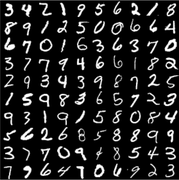
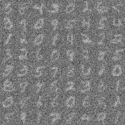
Generative Adversarial Networks operate by simulating complex distributions but training them requires access to large amounts of high quality data. Often times we only have access to noisy or partial observations, from here on referred to as measurements of the true data. If we know the measurement function and would like to train a generative model for the true data, there are several ways to continue | Generative Adversarial Networks operate by simulating complex distributions but training them requires access to large amounts of high quality data. Often times we only have access to noisy or partial observations, which will from here on be referred to as measurements of the true data. If we know the measurement function and would like to train a generative model for the true data, there are several ways to continue which have varying degrees of success. We will use noisy MNIST data as an illustrative example. Suppose we only see MNIST data that has been run through a Gaussian kernel (blurred) with some noise from a <math>N(0, 0.5^2)</math> distribution added to each pixel: | ||
<gallery mode="packed"> | <gallery mode="packed"> | ||
Revision as of 21:09, 5 March 2018
Introduction
Generative Adversarial Networks operate by simulating complex distributions but training them requires access to large amounts of high quality data. Often times we only have access to noisy or partial observations, which will from here on be referred to as measurements of the true data. If we know the measurement function and would like to train a generative model for the true data, there are several ways to continue which have varying degrees of success. We will use noisy MNIST data as an illustrative example. Suppose we only see MNIST data that has been run through a Gaussian kernel (blurred) with some noise from a [math]\displaystyle{ N(0, 0.5^2) }[/math] distribution added to each pixel:
-
True Data (Unobserved)
-
Measured Data (Observed)
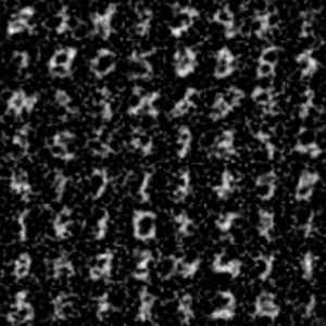
Ignore the problem
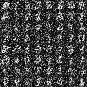
Train a generative model directly on the measured data. This will obviously be unable to generate the true distribution before measurement has occurred.
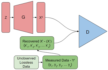
Try to recover the information lost
Works better than ignoring the problem but depends on how easily the measurement function can be inverted.
AmbientGAN
Ashish Bora, Eric Price and Alexandros G. Dimakis propose AmbientGAN as a way to recover the true underlying distribution from measurements of the true data.
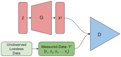
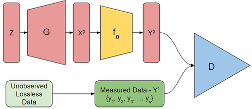
AmbientGAN works by training a generator which attempts to have the measurements of the output it generates fool the discriminator. The discriminator must distinguish between real and generated measurements.
Model
For the following variables superscript [math]\displaystyle{ r }[/math] represents the true distributions while superscript [math]\displaystyle{ g }[/math] represents the generated distributions. Let [math]\displaystyle{ x }[/math], represent the underlying space and [math]\displaystyle{ y }[/math] for the measurement.
Thus [math]\displaystyle{ p_x^r }[/math] is the real underlying distribution over [math]\displaystyle{ \mathbb{R}^n }[/math] that we are interested in. However if we assume our (known) measurement functions, [math]\displaystyle{ f_\theta: \mathbb{R}^n \to \mathbb{R}^m }[/math] are parameterized by [math]\displaystyle{ \theta \sim p_\theta }[/math], we can only observe [math]\displaystyle{ y = f_\theta(x) }[/math].
Mirroring the standard GAN setup we let [math]\displaystyle{ Z \in \mathbb{R}^k, Z \sim p_z }[/math] and [math]\displaystyle{ \Theta \sim p_\theta }[/math] be random variables coming from a distribution that is easy to sample.
If we have a generator [math]\displaystyle{ G: \mathbb{R}^k \to \mathbb{R}^n }[/math] then we can generate [math]\displaystyle{ X^g = G(Z) }[/math] which has distribution [math]\displaystyle{ p_x^g }[/math] a measurement [math]\displaystyle{ Y^g = f_\Theta(G(Z)) }[/math] which has distribution [math]\displaystyle{ p_y^g }[/math].
Unfortunately we do not observe any [math]\displaystyle{ X^g \sim p_x }[/math] so we can use the discriminator directly on [math]\displaystyle{ G(Z) }[/math] to train the generator. Instead we will use the discriminator to distinguish between the [math]\displaystyle{ Y^g - f_\Theta(G(Z)) }[/math] and [math]\displaystyle{ Y^r }[/math]. That is we train the discriminator, [math]\displaystyle{ D: \mathbb{R}^m \to \mathbb{R} }[/math] to detect if a measurement came from [math]\displaystyle{ p_y^r }[/math] or [math]\displaystyle{ p_y^g }[/math].
AmbientGAN has the objective function:
[math]\displaystyle{ \min_G \max_D \mathbb{E}_{Y^r \sim p_y^r}[q(D(Y^r))] + \mathbb{E}_{Z \sim p_z, \Theta \sim p_\theta}[q(1 - D(f_\Theta(G(Z))))] }[/math]
where [math]\displaystyle{ q(.) }[/math] is the quality function; for the standard GAN [math]\displaystyle{ q(x) = log(x) }[/math] and for Wasserstein GAN [math]\displaystyle{ q(x) = x }[/math].
As a technical limitation we require [math]\displaystyle{ f_\theta }[/math] to be differentiable with the respect each input for all values of [math]\displaystyle{ \theta }[/math].
With this set up we sample [math]\displaystyle{ Z \sim p_z }[/math], [math]\displaystyle{ \Theta \sim p_\theta }[/math], and [math]\displaystyle{ Y^r \sim U\{y_1, \cdots, y_s\} }[/math] each iteration and use them to compute the stochastic gradients of the objective function. We alternate between updating [math]\displaystyle{ G }[/math] and updating [math]\displaystyle{ D }[/math].
Empirical Results
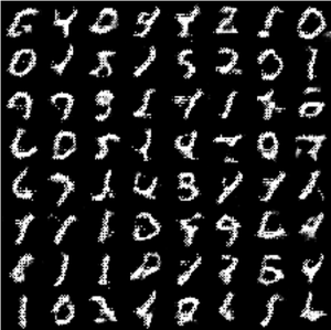
The paper continues to present results of AmbientGAN under various measurement functions when compared to baseline models. We have already seen one example in the introduction: a comparison of AmbientGAN in the Convolve + Noise Measurement case compared to the ignore-baseline, and the unmeasure-baseline.
Block-Pixels
With the block-pixels measurement function each pixel is independently set to 0 with probability [math]\displaystyle{ p }[/math].
Measurements from the celebA dataset with [math]\displaystyle{ p=0.95 }[/math] (left). Images generated from GAN trained on unmeasured (via blurring) data (middle). Results generated from AmbientGAN (right).
Block-Patch
A random 14x14 patch is set to zero (left). Unmeasured using-navier-stoke inpainting (middle). AmbientGAN (right).
Pad-Rotate-Project-[math]\displaystyle{ \theta }[/math]
Results generated by AmbientGAN where the measurement function 0 pads the images, rotates it by [math]\displaystyle{ \theta }[/math], and projects it on to the x axis. For each measurement the value of [math]\displaystyle{ \theta }[/math] is known.
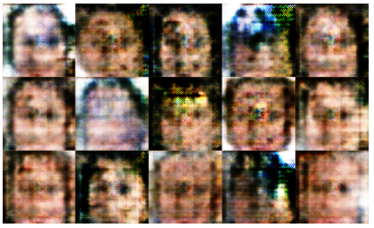
The generated images only have the basic features of a face and is referred to as a failure case in the paper. However the measurement function performs relatively well given how lossy the measurement function is.
MNIST Inception
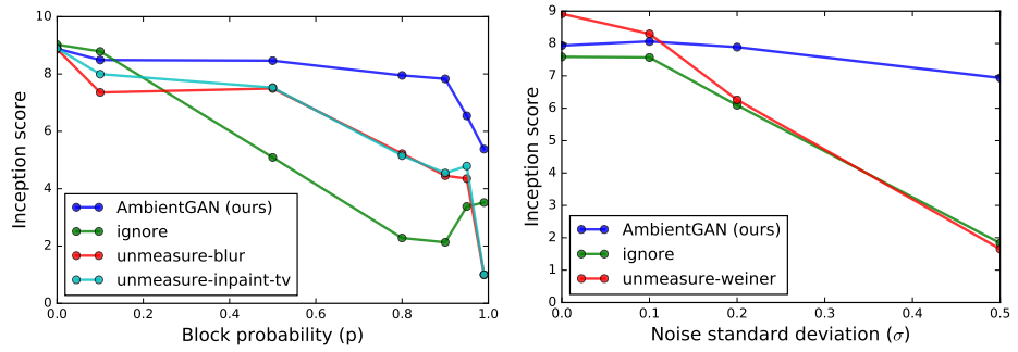
AmbientGAN was compared with baselines through training several models with different probability [math]\displaystyle{ p }[/math] of blocking pixels. The plot on the left shows that the inception scores change as the block probability [math]\displaystyle{ p }[/math] changes. All four models are similar when no pixels are blocked [math]\displaystyle{ (p=0) }[/math]. By the increase of the blocking probability, AmbientGAN models present a relatively stable performance and perform better than the baseline models. Therefore, AmbientGAN is more robust than all other baseline models.
The plot on the right reveals the changes in inception scores while the standard deviation of the additive Gaussian noise increased. Baselines perform better when the noise is small. By the increase of the variance, AmbientGAN models present a much better performance compare to the baseline models. Further AmbientGAN retains high inception scores as measurements become more and more lossy.
CIFAR-10 Inception
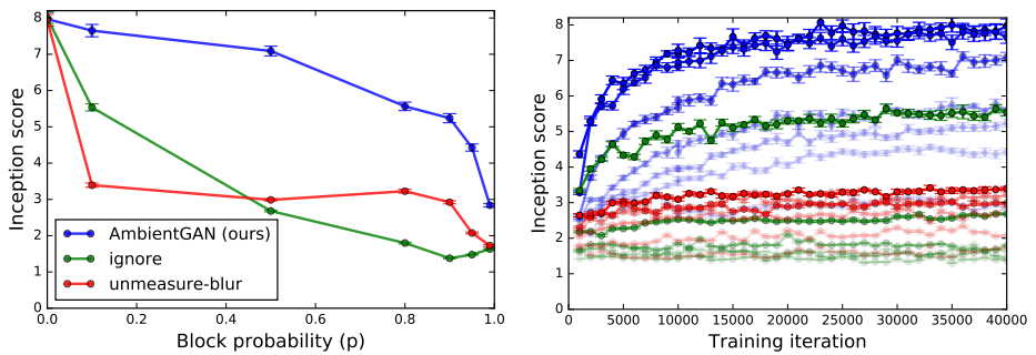
AmbientGAN is faster to train and more robust even on more complex distributions such as CIFAR-10.
Theoretical Results
The theoretical results in the paper prove the true underlying distribution of [math]\displaystyle{ p_x^r }[/math] can be recovered when we have data that comes from the Gaussian-Projection measurement, Fourier transform measurement and the block-pixels measurement. The do this by showing the distribution of the measurements [math]\displaystyle{ p_y^r }[/math] corresponds to a unique distribution [math]\displaystyle{ p_x^r }[/math]. Thus even when the measurement itself is non-invertible the effect of the measurement on the distribution [math]\displaystyle{ p_x^r }[/math] is invertible. Lemma 5.1 ensures this is sufficient to provide the AmbientGAN training process with a consistency guarantee. For full proofs of the results please see appendix A.
Lemma 5.1
Let [math]\displaystyle{ p_x^r }[/math] be the true data distribution, and [math]\displaystyle{ p_\theta }[/math] be the distributions over the parameters of the measurement function. Let [math]\displaystyle{ p_y^r }[/math] be the induced measurement distribution.
Assume for [math]\displaystyle{ p_\theta }[/math] there is a unique probability distribution [math]\displaystyle{ p_x^r }[/math] that induces [math]\displaystyle{ p_y^r }[/math].
Then for the standard GAN model if the Discriminator is optimal, then a generator [math]\displaystyle{ G }[/math] is optimal if and only if [math]\displaystyle{ p_x^g = p_x^r }[/math].
Theorems 5.2
For the Gussian-Projection measurement model, there is a unique underlying distribution [math]\displaystyle{ p_x^{r} }[/math] that can induce the observed measurement distribution [math]\displaystyle{ p_y^{r} }[/math].
Theorems 5.3
Let [math]\displaystyle{ \mathcal{F} (\cdot) }[/math] denote the Fourier transform and let [math]\displaystyle{ supp (\cdot) }[/math] be the support of a function. Consider the Convolve+Noise measurement model with the convolution kernel [math]\displaystyle{ k }[/math]and additive noise distribution [math]\displaystyle{ p_\theta }[/math]. If [math]\displaystyle{ supp( \mathcal{F} (k))^{c}=\phi }[/math] and [math]\displaystyle{ supp( \mathcal{F} (p_\theta))^{c}=\phi }[/math], then there is a unique distribution [math]\displaystyle{ p_x^{r} }[/math] that can induce the measurement distribution [math]\displaystyle{ p_y^{r} }[/math].
Theorems 5.4
Assume that each image pixel takes values in a finite set P. Thus [math]\displaystyle{ x \in P^n \subset \mathbb{R}^{n} }[/math]. Assume [math]\displaystyle{ 0 \in P }[/math], and consider the Block-Pixels measurement model with [math]\displaystyle{ p }[/math] being the probability of blocking a pixel. If [math]\displaystyle{ p \lt 1 }[/math], then there is a unique distribution [math]\displaystyle{ p_x^{r} }[/math] that can induce the measurement distribution [math]\displaystyle{ p_y^{r} }[/math]. Further, for any [math]\displaystyle{ \epsilon \gt 0, \delta \in (0, 1] }[/math], given a dataset of \begin{equation} s=\Omega \left( \frac{|P|^{2n}}{(1-p)^{2n} \epsilon^{2}} log \left( \frac{|P|^{n}}{\delta} \right) \right) \end{equation} IID measurement samples from pry , if the discriminator D is optimal, then with probability [math]\displaystyle{ \geq 1 - \delta }[/math] over the dataset, any optimal generator G must satisfy [math]\displaystyle{ d_{TV} \left( p^g_x , p^r_x \right) \leq \epsilon }[/math], where [math]\displaystyle{ d_{TV} \left( \cdot, \cdot \right) }[/math] is the total variation distance.
Future Research
One critical weakness of AmbientGAN is the assumption that the measurement model is known. It would be nice to be able to train an AmbientGAN model when we have an unknown measurement model but also a small sample of unmeasured data.
