Unsupervised Domain Adaptation with Residual Transfer Networks

Introduction

Domain Adaptation [1]is a problem in machine learning which involves taking a model which has been trained on a source domain, and applying this to a different (but related) target domain. Unsupervised domain adaptation refers to the situation in which the source data is labelled, while the target data is (predominantly) unlabeled. The problem at hand is then finding ways to generalize the learning on the source domain to the target domain. In the age of deep networks this problem has become particularly salient due to the need for vast amounts of labeled training data, in order to reap the benefits of deep learning. Manual generation of labeled data is often prohibitive, and in absence of such data networks are rarely performant. The attempt to circumvent this drought of data typically necessitates the gathering of "off-the-shelf" data sets, which are tangentially related and contain labels, and then building models in these domains. The fundamental issue that unsupervised domain adaptation attempts to address is overcoming the inherent shift in distribution across the domains, without the ability to observe this shift directly.

This paper proposes a method for unsupervised domain adaptation which relies on three key components:

1. A kernel-based penalty to ensure that the abstract representations generated by the networks hidden layers are similar between the source and the target data;
2. An entropy based penalty on the target classifier, which exploits the entropy minimization principle; and
3. A residual network structure is appended, which allows the source and target classifiers to differ by a (learned) residual function, thus relaxing the shared classifier assumption which is traditionally made.

This method outperforms state-of-the-art techniques on common benchmark datasets, and is flexible enough to be applied in most feed-forward neural networks.

The Office-31 Dataset Images for Backpack. Shows the variation in the source and target domains to motivate why these methods are important.

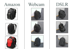
Working Example (Office-31)

In order to assist in the understanding of the methods, it is helpful to have a tangible sense of the problem front of mind. The Domain Adaptation Project [2] provides data sets which are tailored to the problem of unsupervised domain adaptation. One of these data sets (which is later used in the experiments of this paper) has images which are labeled based on the Amazon product page for the various items. There are then corresponding pictures taken either by webcams or digital SLR cameras. The goal of unsupervised domain adaptation on this data set would be to take any of the three image sources as the source domain, and transfer a classifier to the other domain; see the example images to understand the differences.

One can imagine that, while it is likely easy to scrape labeled images from Amazon, it is likely far more difficult to collect labeled images from webcam or DSLR pictures directly. The ultimate goal of this method would be to train a model to recognize a picture of a backpack taken with a webcam, based on images of backpacks scraped from Amazon (or similar tasks).

Related Work

Broadly speaking, the problem of domain adaptation mitigates manual labeling of data in areas such as machine learning, computer vision, and natural language processing. The general goal of domain adaptation is to reduce the discrepancy in probability distributions between the source and target domains.

Research into the use of Deep Neural Networks for the purpose of domain adaptation has suggested that, while networks learn abstract feature representations which can reduce the discrepancy across domains, it is not possible to wholly remove it [3], [4]. Further work has been done to design networks which adapt traditional deep nets (typically CNNs) to specifically address the problems posed by domain adaptation, these methods all only address the issue of feature adaptation [5], [6], [7]. That is, they all assume that the target and source classifiers are shared between domains.

The authors drew particular motivation from He et al. [8] with the proposed structure of residual networks. Combining the insights from the ResNet architecture, in addition to previous work that had leveraged classifier adaptation (in the context where some target data is labeled) [9], [10], [11] the authors develop their proposed network.

Residual Transfer Networks

Generally, in an unsupervised domain adaptation problem, we are dealing with a set $\mathcal{D}_s$ (called the source domain) which is defined by $\{(x_i^s, y_i^s)\}_{i=1}^{n_s}$. That is the set of all labeled input-output pairs in our source data set. We denote the number of source elements by $n_s$. There is a corresponding set $\mathcal{D}_t = \{(x_i^t)\}_{i=1}^{n_t}$ (the target domain), consisting of unlabeled input values. There are $n_t$ such values.

The overarching structure of the RTN. Consists of an existing network, to which a bottleneck, MMD block, and residual block is appended.

We can think of $\mathcal{D}_s$ as being sampled from some underlying distribution $p$, and $\mathcal{D}_t$ as being sampled from $q$. Generally we have that $p \neq q$, partially motivating the need for domain adaptation methods.

We can consider the classifiers $f_s(\underline{x})$ and $f_t(\underline{x})$, for the source domain and target domain respectively. It is possible to learn $f_s$ based on the sample $\mathcal{D}_s$. Under the shared classifier assumption it would be the case that $f_s(\underline{x}) = f_t(\underline{x})$, and thus learning the source classifier is enough. This method relaxes this assumption, assuming that in general $f_s \neq f_t$, and attempting to learn both.

The example network extends deep convolutional networks (in this case AlexNet [12]) to Residual Transfer Networks, the mechanics of which are outlined below. Recall that, if $L(\cdot, \cdot)$ is taken to be the cross-entropy loss function, then the empirical error of a CNN on the source domain $\mathcal{D}_s$ is given by:

[math]\displaystyle{ \min_{f_s} \frac{1}{n_s} \sum_{i=1}^{n_s} L(f_s(x_i^s), y_i^s) }[/math]

In a standard implementation, the CNN optimizes over the above loss. This will be the starting point for the RTN.

Structural Overview

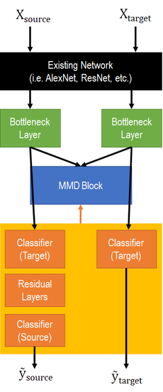
The model proposed in this paper extends existing CNN's and alters the loss function that is optimized over. While each of these components is discussed in depth below, the overarching architecture involves four components:

1. An existing deep model. While this can be any model, in theory, the authors leverage AlexNet in practice.
2. A bottleneck layer, used to reduce the dimensionality of the learned abstract feature space, directly after the existing network.
3. An MMD block, with the expressed intention of feature adaptation.
4. A residual block, with the expressed intention of classifier adaptation.

This structure is then optimized against a loss function which combines the standard cross-entropy penalty with MMD and target entropy penalties, yielding the proposed Residual Transfer Network (RTN) structure.

Feature Adaptation

Feature adaptation refers to the process in which the features which are learned to represent the source domain are made applicable to the target domain. Broadly speaking a CNN works to generate abstract feature representations of the distribution that the inputs are sampled from. It has been found that using these deep features can reduce, but not remove, cross-domain distribution discrepancy, hence the need for feature adaptation. It is important to note that CNN's transfer from general to specific features as the network gets deeper. In this light, the discrepancy between the feature representation of the source and the target will grow through a deeper convolutional net. As such a technique for forcing these distributions to be similar is needed.

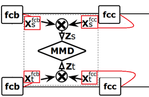
In particular the authors of this paper impose a bottleneck layer (call it $fc_b$) which is included after the final convolutional layer of AlexNet. This dense layer is connected to an additional dense layer $fc_c$, (which will serve as the target classification layer). They then compute the tensor product between the activations of the layers, performing "lossless multi-layer feature fusion". That is for the source domain they define $z_i^s \overset{\underset{\mathrm{def}}{}}{=} x_i^{s,fc_b}\otimes x_i^{s,fc_c}$ and for the target domain, $z_i^t \overset{\underset{\mathrm{def}}{}}{=} x_i^{t,fc_b}\otimes x_i^{t,fc_c}$. The authors then employ feature adaptation by means of Maximum Mean Discrepancy, between the source and target domains, on these fusion features.

The Maximum Mean Discrepancy Block (MMD) included in the RTN. The outputs of $fc_b$ and $fc_c$ are fused through a tensor product, and then passed through the MMD penalty, ensuring distributional similarity.

Maximum Mean Discrepancy

The Maximum Mean Discrepancy (MMD) is a Kernel method involes mapping to a Reproducing Kernel Hilbert Space (RKHS) [13]. Denote the RKHS $\mathcal{H}_K$ with a characteristic kernel $K$. We then define the mean embedding of a distribution $p$ in $\mathcal{H}_K$ to be the unique element $\mu_K(p)$ such that $\mathbf{E}_{x\sim p}f(x) = \langle f(x), \mu_K(p)\rangle_{\mathcal{H}_K}$ for all $f \in \mathcal{H}_K$. Now, if we take $\phi: \mathcal{X} \to \mathcal{H}_K$, then we can define the MMD between two distributions $p$ and $q$ as follows:

[math]\displaystyle{ d_k(p, q) \overset{\underset{\mathrm{def}}{}}{=} ||\mathbf{E}_{x\sim p}(\phi(x^s)) - \mathbf{E}_{x\sim q}(\phi(x^t))||_{\mathcal{H}_K} }[/math]

Effectively, the MMD will compute the self-similarity of $p$ and $q$, and subtract twice the cross-similarity between the distributions: $\widehat{\text{MMD}}^2 = \text{mean}(K_{pp}) + \text{mean}(K_{qq}) - 2\times\text{mean}(K_{pq})$. From here we can infer that $p$ and $q$ are equivalent distributions if and only if the $\text{MMD} = 0$. If we then wish to force two distributions to be similar, this becomes a minimization problem over the MMD.

Two important notes:

1. The RKHS, and as such MMD, depend on the choice of the kernel;
2. Computing the MMD efficiently requires an unbiased estimate of the MMD (as outlined [14]).

MMD for Feature Adaptation in the RTN

The authors wish to minimize the MMD between the fusion features outlined above derived from the source and target domains. Concretely this amounts to forcing the distribution of the abstract representation of the source domain $\mathcal{D}_s$ to be similar to the distribution of the abstract representation of the target domain $\mathcal{D}_t$. Performing this optimization over the fused features between the $fb_b$ and $fb_c$ forces each of those layers towards similar distributions.

Practically this involves an additional penalty function given by the following:

[math]\displaystyle{ D_{\mathcal{L}}(\mathcal{D}_s, \mathcal{D}_t) = \sum_{i,j=1}^{n_s} \frac{k(z_i^s, z_j^s)}{n_s^2} + \sum_{i,j=1}^{n_t} \frac{k(z_i^t, z_j^t)}{n_t^2} + \sum_{i=1}^{n_s}\sum_{j=1}^{n_t} \frac{k(z_i^s, z_j^t)}{n_sn_t} }[/math]

Where the characteristic kernel $k(z, z')$ is the Gaussian kernel, defined on the vectorization of tensors, with bandwidth parameter $b$. That is: $k(z, z') = \exp(-||vec(z) - vec(z')||^2/b)$.

Classifier Adaptation

In traditional unsupervised domain adaptation there is a shared-classifier assumption which is made. In essence, if $f_s(x)$ represents the classifier on the source domain, and $f_t(x)$ represents the classifier on the target domain then this assumption simply states that $f_s = f_t$. While this may seem to be a reasonable assumption at first glance, it is problematic largely in that this is an assumption that is incredibly difficult to check. If it could be readily confirmed that the source and target classifiers could be shared, then the problem of domain adaptation would be largely trivialized. Instead, the authors here relax this assumption slightly. They postulate that instead of being equivalent, the source and target classifier differ by some perturbation function $\Delta f$. The general idea is that, by assuming $f_S(x) = f_T(x) + \Delta f(x)$, where $f_S$ and $f_T$ correspond to the source and target classifiers, pre-activation, and $\Delta f(x)$ is some residual function.

The authors then suggest using residual blocks, as popularized by the ResNet framework [15], to learn this residual function.

A comparison of a standard Deep Neural Network block which is designed to fit a function H(x) compared to a residual block which fits H(x) as the sum of the input, x, and a learned residual function, F(X).

Residual Networks Framework

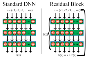
A (Deep) Residual Network, as proposed initially in ResNet, employs residual blocks to assist in the learning process, and were a key component of being able to train extraordinarily deep networks. The Residual Network is comprised largely in the same manner as standard neural networks, with one key difference, namely the inclusion of residual blocks - sets of layers which aim to estimate a residual function in place of estimating the function itself.

That is, if we wish to use a DNN to estimate some function $h(x)$, a residual block will decompose this to $h(x) = F(x) + x$. The layers are then used to learn $F(x)$, and after the layers which aim to learn this residual function, the input $x$ is recombined through element-wise addition, to form $h(x) = F(x) + x$. This was initially proposed as a manner to allow for deeper networks to be effectively trained, but has since used in novel contexts.

Residual Blocks in the RTN

The Structure of the Residual Block in the RTN framework. The block relies on two additional dense layers following the target classifier in an attempt to learn the residual difference between the source and target classifiers.

The authors leverage residual blocks for the purpose of classifier adaptation. Operating under the assumption that the source and target classifiers differ by an arbitrary perturbation function, $f(x)$, the authors add an additional set of densely connected layers which the source data will flow through. In particular, the authors take the $fc_c$ layer above as the desired target classifier. For the source data an additional set of layers ($fc-1$ and $fc-2$) are added following $fc_c$, which are connected as a residual block. The output of the classifier layer is then added back to the output of the residual block in order to form the source classifier.

It is necessary to note that in this case the output from $fc_c$ passes the non-activated (i.e. pre-softmax activation) to the element-wise addition, the result of which is passed through the activation layer, yielding the source prediction. In the provided diagram, we have that $f_S(x)$ represents the non-activated output from the additive layer in the residual block; $f_T(x)$ represents the non-activated output from the target classifier; and $fc-1$/$fc-2$ are used to learn the perturbation function $\Delta f(x)$.

Entropy Minimization

In addition to the residual blocks, the authors make use of the entropy minimization principle [16] to further refine the classifier adaptation. In particular, by minimizing the entropy of the target classifier (or more correctly, the entropy of the class conditional distribution $f_j^t(x_i^t) = p(y_i^t = j \mid x_i^t; f_t)$), low-density separation between the classes is encouraged. Low-Density Separation is a concept used predominantly in semi-supervised learning, which in essence tries to draw class decision boundaries in regions where there are few data points (labeled or unlabeled). The above paper leverages an entropy regularization scheme to achieve the goal low-density separation goal; this is adopted here to the case of unsupervised domain adaptation.

In practice this amounts to adding a further penalty based on the entropy of the class conditional distribution. In particular, if $H(\cdot)$ is defined to be the entropy function, such that $H(f_t(x_i^t)) = - \sum_{j=1}^c f_j^t(x_i^t)\log f_j^t(x_i^t)$, where $c$ is the number of classes and $f_j^t(x_i^t)$ represents the probability of predicting class $j$ for point $x_i^t$, then over the target domain $\mathcal{D}_t$ we define the entropy penalty to be:

[math]\displaystyle{ \frac{1}{n_t} \sum_{i=1}^{n_t} H(f_t(x_i^t)) }[/math]

The combination of the residual learning and the entropy penalty, the authors hypothesize will enable effective classifier adaptation.

Residual Transfer Network

The combination of the MMD loss introduced in feature adaptation, the residual block introduced in classifier adaptation, and the application of the entropy minimization principle cumulates in the Residual Transfer Network proposed by the authors. The model will be optimized according to the following loss function, which combines the standard cross-entropy, MMD penalty, and entropy penalty:

[math]\displaystyle{ \min_{f_s = f_t + \Delta f} \underbrace{\left(\frac{1}{n_s} \sum_{i=1}^{n_s} L(f_s(x_i^s), y_i^s)\right)}_{\text{Typical Cross-Entropy}} + \underbrace{\frac{\gamma}{n_t}\left(\sum_{i=1}^{n_t} H(f_t(x_i^t)) \right)}_{\text{Target Entropy Minimization}} + \underbrace{\lambda\left(D_{\mathcal{L}}(\mathcal{D}_s, \mathcal{D}_t)\right)}_{\text{MMD Penalty}} }[/math]

Where we take $\gamma$ and $\lambda$ to be tradeoff parameters between the entropy penalty and the MMD penalty.

The full network, which is trained subject to the above optimization problem, thus takes on the following structure.

Experiments

Set-up

The performance of RTN was jointly compared across two key data sets in the area of Unsupervised Domain Adaptation. Specifically, Office-31 (discussed in the introduction) and Office-Caltech (maintained by the same project group). Office-31 is comprised of images from 3 sources, Amazon (A), Webcam (W), and DSLR (D), of 31 different objects. Office-Caltech is derived by considering 10 classes common to both the Office-31 and the Caltech data sets, thus providing further adaptation possibilities. This provides 6 Transfer Tasks on the 31 classes of Office-31 ($\{(A,W), (A,D), (W,A), (W,D), (D,A), (D,W)\}$) and 12 Transfer Tasks on the 10 classes of Office-Caltech ($\{(A,W), (A,D), (A,C), (W,A), (W,D), (W,C), (D,A), (D,W), (D,C), (C,A), (C,W), (C,D)\}$).

The authors then compare the results on the 18 different adaptation tasks against 6 other models. In order to determine the efficacy of the various contributions outlined in the paper they perform an ablation study, evaluating variants of the RTN. Specifically, they consider the RTN with only the MMD module (RTN (mmd)), the RTN with the MMD module and the entropy minimization (RTN (mmd+ent)), and the complete RTN (RTN (mmd+ent+res)). The experiments leverage all the labeled training data and compute accuracy across all unlabeled domain data. The parameters of the model (i.e. $\gamma$, and $\lambda$) are fixed based on a single validation point on the transfer task $\mathbf{A}\to\mathbf{W}$. These parameters are then maintained across all transfer tasks.

As for specification details, the authors use mini-batch SGD, with momentum $0.9$, and with the learning rate adjusted based on $\eta_p = \frac{\eta_0}{(1 + \alpha p)^\beta}$, where $p$ indicates the portion of training completed (linear from $0$ to $1$), $\eta_0 = 0.01$, $\alpha = 10$ and $\beta = 0.75$, which was optimized for low error on the source. The MMD and entropy parameters, set as above, were maintained at $\lambda = 0.3$ and $\gamma - 0.3$.

Results

Results from the Office-31 Experiment

Results from the Office-Caltech Experiment

In aggregate, the network outperformed all comparison methods, across all transfer tasks. Broadly speaking the network saw the largest increases in accuracy on the hard transfer tasks (for instance $\mathbf{A} \to \mathbf{C}$), where the source-domain discrepancy is large. The authors take this to mean that the proposed model learns "more adaptive classifiers and transferable features for safer domain adaptation." They further indicate that standard deep learning techniques (i.e. just AlexNet) perform similarly to standard shallow techniques (TCA and GFK). Deep-transfer methods which focus on feature adaptation perform significantly better than the standard methods. The proposed RTN, which adds in additional considerations for classifier adaptation, performs even better.

In addition, the ablation study found a number of interesting results:

1. The RTN (mmd) outperforms DAN, which is founded on a similar method, but contains multiple MMD penalties (one for each layer instead of on a bottleneck), and is as such less computationally efficient;
2. The addition of the entropy penalty [RTN (mmd+ent)] provides significant marginal benefit over the previous RTN (mmd);
3. The full RTN [RTN (mmd+ent+res)] performs the best of all variants, by diminishing returns are seen over the addition of the entropy penalty.

Overall the authors claim that the RTN (mmd+ent+res) is now regarded as state-of-the-art for unsupervised domain adaptation.

Discussion

t-SNE Embeddings Comparing the Performance of DAN and RTN

The Mean and Standard Deviations of the outputs from the Source Classifier, Target Classifier, and Residual Functions. As expected, the residual function provides a small, but non-zero, contribution.

The accuracy of tests by varying the parameter $\gamma$. We first see an increase in accuracy up to an ideal point, before having the accuracy fall again.

The corresponding weights of the classifier layers, if trained on the labeled source and target data, exhibiting the differences which exist between the two classifiers in an ideal state.

Visualizing Predictions (Versus DAN)

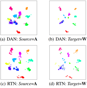
DAN uses a similar method for feature adaptation but neglects any attempt at classifier adaptation (i.e. it makes the shared-classifier assumption). In order to demonstrate that this leads to the worse performance, the authors provide images showing the t-SNE embeddings by DAN and RTN on the transfer task $\mathbf{A} \to \mathbf{W}$. The images show that the target categories are not well discriminated by the source classifier, suggesting a violation of the shared-classifier assumption. Conversely, the target classifier for the RTN exhibits better discrimination.

Layer Responses and Classifier Shift

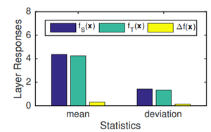
The authors further consider the mean and standard deviation of the outputs of $f_S(x)$, $f_T(x)$ and $\Delta f(x)$ to consider the relative contributions of the different components. As expected, $\Delta f(x)$ provides a small (though non-zero) contribution to the learned source classifier. This provides some merit to the idea of residual learning on the classifiers.

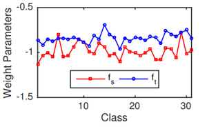
In addition, the authors train classifiers on the source and target data, with labels present, and compare the realized weights. This is used to test how different the ideal weights are on separate classifiers. The results suggest that there is, in fact, a discrepancy between the classifiers, further motivating the use of tactics to avoid the shared-classifier assumption.

Parameter Sensitivity

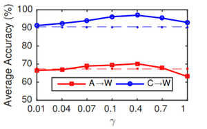
Lastly, the authors test the sensitivity of these results against the parameter $\gamma$. They run this test on $\mathbf{A}\to\mathbf{W}$ in addition to $\mathbf{C}\to\mathbf{W}$, varying the parameter from $0.01$ to $1.0$. They find that, on both tasks, the increase of the parameter initially improves accuracy, before seeing a drop-off.

Conclusion

This paper presented a novel approach to unsupervised domain adaptation which relaxed assumptions made by previous models with regard to the shared nature of classifiers. Like previous models this proposed network leverages feature adaptation by matching the distributions of features across the domains. In addition, using a residual network and entropy minimization tactic, the target classifier is allowed to differ from the source classifier. In particular, this approach allows for easy integration into existing networks, and can be implemented with any standard deep learning software.

For follow-up considerations, the authors propose looking for adaptations which may be useful in the semi-supervised domain adaptation problem.

Critique

While the paper presents a clear approach, which empirically attains great results on the desired tasks, I question the benefit to the residual block that is employed. The results of the ablation study seem to suggest that the majority of the benefits can be derived from using the MMD and Entropy penalties. The residual block appears to add marginal, perhaps insignificant contributions to the outcome. Despite this, the use of MMD loss is not novel, and the entropy loss is less well documented, and less thoroughly explored. Perhaps a different set of ablations would have indicated that the three parts, indeed, are equally effective (and the diminishing returns stems from stacking the three methods), but as it is presented, I question the utility of the final structure versus a less complicated, less novel approach.

References

1. https://en.wikipedia.org/wiki/Domain_adaptation
2. https://people.eecs.berkeley.edu/~jhoffman/domainadapt/