Deep Exploration via Bootstrapped DQN: Difference between revisions
Ashishgaurav (talk | contribs) (edited summary a bit) |
Ashishgaurav (talk | contribs) (→Gist) |
||
| Line 1: | Line 1: | ||
== | === Status: In Progress === | ||
== Intro to Reinforcement Learning == | |||
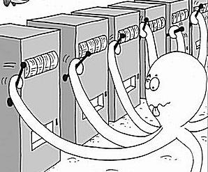
In reinforcement learning, an agent interacts with an environment with the goal to maximize its long term reward. This is the same as [https://en.wikipedia.org/wiki/Multi-armed_bandit multi armed bandit problem]. In a multi armed bandit problem, there is a gambler and there are $n$ slot machines, and the gambler can choose to play any specific slot machine at any time. All the slot machines have their own probability distributions by which they churn out rewards, but this is unknown to the gambler. So the question is, how can the gambler learn how to get the maximum long term reward? | |||
There are two things the gambler can do at any instance: either he can try a new slot machine, or he can play the slot machine he has tried before (and he knows he will get some reward). However, even though trying a new slot machine feels like it would bring less reward to the gambler, it is possible that the gambler finds out a new slot machine that gives a better reward than the current best slot machine. This is the dilemma of '''exploration vs exploitation'''. Trying out a new slot machine is '''exploration''', while redoing the best move so far is '''exploiting''' the currently understood perception of the reward. | |||
[[File:multiarmedbandit.jpg|thumb|Source: [https://blogs.mathworks.com/images/loren/2016/multiarmedbandit.jpg blogs.mathworks.com]]] | |||
There are many strategies to approach this '''exploration-exploitation dilemma'''. A simple list of strategies can be found online [https://web.stanford.edu/class/msande338/lec9.pdf here]. A lot of these approaches are provably efficient, but assume that the state space is not very large. Strategies for large state spaces often just either ignore exploration, or do something naive like $\epsilon$-greedy, where you exploit with $1-\epsilon$ probability and explore "randomly" in rest of the cases. | |||
This paper tries to use a Thompson sampling like approach to make decisions. | |||
== Thompson Sampling<sup>[[#References|[1]]]</sup> == | |||
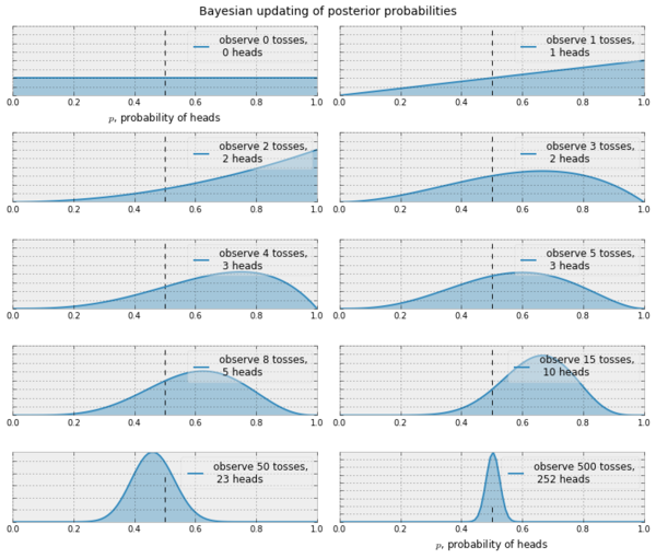
In Thompson sampling, our goal is to reach a belief that resembles the truth. Let's consider a case of coin tosses (2-armed bandit). Suppose we want to be able to reach a satisfactory pdf for $\mathbb{P}_h$ (heads). Assuming that this is a Bernoulli bandit problem, i.e. the rewards are $0$ or $1$, we can start off with $\mathbb{P}_h^{(0)}=\beta(1,1)$. The $\beta(x,y)$ distribution is a very good choice for a possible pdf because it works well for Bernoulli rewards. Further $\beta(1,1)$ is the uniform distribution $\mathbb{N}(0,1)$. | |||
Now, at every iteration $t$, we observe the reward $R^{(t)}$ and try to make our belief close to the truth by doing a Bayesian computation. Assuming $p$ is the probability of getting a heads, | |||
$$ | |||
\begin{align*} | |||
\mathbb{P}(R|D) &\propto \mathbb{P}(D|R) \cdot \mathbb{P}(R) \\ | |||
\mathbb{P}_h^{(t+1)}&\propto \mbox{likelihood}\cdot\mbox{prior} \\ | |||
&\propto p^{R^{(t)}}(1-p)^{R^{(t)}} \cdot \mathbb{P}_h^{(t)} \\ | |||
&\propto p^{R^{(t)}}(1-p)^{R^{(t)}} \cdot \beta(x_t, y_t) \\ | |||
&\propto p^{R^{(t)}}(1-p)^{R^{(t)}} \cdot p^{x_t-1}(1-p)^{y_t-1} \\ | |||
&\propto p^{x_t+R^{(t)}-1}(1-p)^{y_t+R^{(t)}-1} \\ | |||
&\propto \beta(x_t+R^{(t)}, y_t+R^{(t)}) | |||
\end{align*} | |||
$$ | |||
[[File:thompson sampling coin example.png|thumb||||600px|Source: [https://www.quora.com/What-is-Thompson-sampling-in-laymans-terms Quora]]] | |||
This means that with successive sampling, our belief can become better at approximating the truth. There are similar update rules if we use a non Bernoulli setting, say, Gaussian. In the Gaussian case, we start with $\mathbb{P}_h^{(0)}=\mathbb{N}(0,1)$ and given that $\mathbb{P}_h^{(t)}\propto\mathbb{N}(\mu, \sigma)$ it is possible to show that the update rule looks like | |||
$$ | |||
\mathbb{P}_h^{(t+1)} \propto \mathbb{N}\bigg(\frac{t\mu+R^{(t)}}{t+1},\frac{\sigma}{\sigma+1}\bigg) | |||
$$ | |||
=== How can we use this in reinforcement learning? === | |||
We can use this idea to decide when to explore and when to exploit. We start with an initial belief, choose an action, observe the reward and based on the kind of reward, we update our belief about what action to choose next. | |||
== References == | |||
1. [https://bandits.wikischolars.columbia.edu/file/view/Lecture+4.pdf Learning and optimization for sequential decision making, Columbia University, Lec 4] | |||
Revision as of 20:26, 15 November 2017
Status: In Progress
Intro to Reinforcement Learning
In reinforcement learning, an agent interacts with an environment with the goal to maximize its long term reward. This is the same as multi armed bandit problem. In a multi armed bandit problem, there is a gambler and there are $n$ slot machines, and the gambler can choose to play any specific slot machine at any time. All the slot machines have their own probability distributions by which they churn out rewards, but this is unknown to the gambler. So the question is, how can the gambler learn how to get the maximum long term reward?
There are two things the gambler can do at any instance: either he can try a new slot machine, or he can play the slot machine he has tried before (and he knows he will get some reward). However, even though trying a new slot machine feels like it would bring less reward to the gambler, it is possible that the gambler finds out a new slot machine that gives a better reward than the current best slot machine. This is the dilemma of exploration vs exploitation. Trying out a new slot machine is exploration, while redoing the best move so far is exploiting the currently understood perception of the reward.

There are many strategies to approach this exploration-exploitation dilemma. A simple list of strategies can be found online here. A lot of these approaches are provably efficient, but assume that the state space is not very large. Strategies for large state spaces often just either ignore exploration, or do something naive like $\epsilon$-greedy, where you exploit with $1-\epsilon$ probability and explore "randomly" in rest of the cases.
This paper tries to use a Thompson sampling like approach to make decisions.
Thompson Sampling[1]
In Thompson sampling, our goal is to reach a belief that resembles the truth. Let's consider a case of coin tosses (2-armed bandit). Suppose we want to be able to reach a satisfactory pdf for $\mathbb{P}_h$ (heads). Assuming that this is a Bernoulli bandit problem, i.e. the rewards are $0$ or $1$, we can start off with $\mathbb{P}_h^{(0)}=\beta(1,1)$. The $\beta(x,y)$ distribution is a very good choice for a possible pdf because it works well for Bernoulli rewards. Further $\beta(1,1)$ is the uniform distribution $\mathbb{N}(0,1)$.
Now, at every iteration $t$, we observe the reward $R^{(t)}$ and try to make our belief close to the truth by doing a Bayesian computation. Assuming $p$ is the probability of getting a heads,
$$ \begin{align*} \mathbb{P}(R|D) &\propto \mathbb{P}(D|R) \cdot \mathbb{P}(R) \\ \mathbb{P}_h^{(t+1)}&\propto \mbox{likelihood}\cdot\mbox{prior} \\ &\propto p^{R^{(t)}}(1-p)^{R^{(t)}} \cdot \mathbb{P}_h^{(t)} \\ &\propto p^{R^{(t)}}(1-p)^{R^{(t)}} \cdot \beta(x_t, y_t) \\ &\propto p^{R^{(t)}}(1-p)^{R^{(t)}} \cdot p^{x_t-1}(1-p)^{y_t-1} \\ &\propto p^{x_t+R^{(t)}-1}(1-p)^{y_t+R^{(t)}-1} \\ &\propto \beta(x_t+R^{(t)}, y_t+R^{(t)}) \end{align*} $$

This means that with successive sampling, our belief can become better at approximating the truth. There are similar update rules if we use a non Bernoulli setting, say, Gaussian. In the Gaussian case, we start with $\mathbb{P}_h^{(0)}=\mathbb{N}(0,1)$ and given that $\mathbb{P}_h^{(t)}\propto\mathbb{N}(\mu, \sigma)$ it is possible to show that the update rule looks like
$$ \mathbb{P}_h^{(t+1)} \propto \mathbb{N}\bigg(\frac{t\mu+R^{(t)}}{t+1},\frac{\sigma}{\sigma+1}\bigg) $$
How can we use this in reinforcement learning?
We can use this idea to decide when to explore and when to exploit. We start with an initial belief, choose an action, observe the reward and based on the kind of reward, we update our belief about what action to choose next.
References
1. Learning and optimization for sequential decision making, Columbia University, Lec 4