imageNet Classification with Deep Convolutional Neural Networks

Introduction

In this paper, they trained a large, deep neural network to classify the 1.2 million high-resolution images in the ImageNet LSVRC-2010 contest into the 1000 different classes. To learn about thousands of objects from millions of images, Convolutional Neural Network (CNN) is utilized due to its large learning capacity, fewer connections and parameters and outstanding performance on image classification.

Moreover, current GPU provides a powerful tool to facilitate the training of interestingly-large CNNs. Thus, they trained one of the largest convolutional neural networks to date on the datasets of ILSVRC-2010 and ILSVRC-2012 and achieved the best results ever reported on these datasets by the time this paper was written.

The code of their work is available here<ref> "High-performance C++/CUDA implementation of convolutional neural networks" </ref>.

Dataset

ImageNet Large-Scale Visual Recognition Challenge (ILSVRC) has roughly 1.2 million labeled high-resolution training images, 50 thousand validation images, and 150 thousand testing images over 1000 categories.

In this paper, the images in this dataset are down-sampled to a fixed resolution of 256 x 256. The only image pre-processing they used is subtracting the mean activity over the training set from each pixel.

Architecture

ReLU Nonlinearity

They use Rectified Linear Units (ReLUs)<ref> Nair V, Hinton G E. Rectified linear units improve restricted boltzmann machines. Proceedings of the 27th International Conference on Machine Learning (ICML-10). 2010: 807-814. </ref> as the nonlinearity function, which work several times faster than equivalents with those standard saturating neurons. Thus, better performance can be achieved by reducing the training time for each epoch and training larger datasets to prevent overfitting. Deep convolutional neural networks with ReLUs train several times faster than their equivalents with tanh units. The following figure illustrates this. The shows the number of iterations required to reach 25% training error on the CIFAR-10 dataset for a particular four-layer convolutional network.

A four-layer convolutional neural network with ReLUs (solid line) reaches a 25% training error rate on CIFAR-10 six times faster than an equivalent network with tanh neurons (dashed line). The learning rates for each network were chosen independently to make training as fast as possible. No regularization of any kind was employed. The magnitude of the effect demonstrated here varies with network architecture, but networks with ReLUs consistently learn several times faster than equivalents with saturating neurons.

Training on Multiple GPUs

They spread the net across two GPUs by putting half of the kernels (or neurons) on each GPU and letting GPUs communicate only in certain layers. Choosing the pattern of connectivity could be a problem for cross-validation, so they tune the amount of communication precisely until it is an acceptable fraction of the amount of computation.

Local Response Normalization

ReLUs have the desirable property that they do not require input normalization to prevent them from saturating. However, they find that a local response normalization scheme after applying the ReLU nonlinearity can reduce their top-1 and top-5 error rates by 1.4% and 1.2%.

The response normalization is given by the expression

[math]\displaystyle{ b_{x,y}^{i}=a_{x,y}^{i}/\left ( k+\alpha \sum_{j=max\left ( 0,i-n/2 \right )}^{min\left ( N-1,i+n/2 \right )}\left ( a_{x,y}^{i} \right )^{2} \right )^{\beta } }[/math]

where the sum runs over n “adjacent” kernel maps at the same spatial position. This response normalization implements a form of lateral inhibition inspired by the type found in real neurons, creating competition for big activities amongst neuron outputs computed using different kernels.

Overlapping Pooling

Unlike traditional non-overlapping pooling, they use overlapping pooling throughout their network, with pooling window size z = 3 and stride s = 2. This scheme reduces their top-1 and top-5 error rates by 0.4% and 0.3% and makes the network more difficult to overfit.

Overall Architecture

File:network.JPG

As shown in the figure above, the net contains eight layers with 60 million parameters; the first five are convolutional and the remaining three are fully connected layers. The output of the last layer is fed to a 1000-way softmax. Their network maximizes the average across training cases of the log-probability of the correct label under the prediction distribution.

Response-normalization layers follow the first and second convolutional layers. Max-pooling layers follow both response-normalization layers as well as the fifth convolutional layer. The ReLU non-linearity is applied to the output of every convolutional and fully-connected layer.

Reducing overfitting

Data Augmentation

The easiest and most common method to reduce overfitting on image data is to artificially enlarge the dataset using label-preserving transformations. In this paper, the transformed images are generated on CPU while GPU is training and do not need to be stored on disk.

The first form of data augmentation consists of generating image translations and horizontal reflections. They extract a random 224 x 224 patches (and their horizontal reflections) from the 256 x 256 images and training the network on these extracted patches. They also perform principal components analysis (PCA) on the set of RGB pixel values. To each training image, multiples of the found principal components, with magnitudes proportional to the corresponding eigenvalues times a random variable drawn from a Gaussian with mean zero and standard deviation 0.1 are added.Therefore to each RGB image pixel the following quantity is added

This scheme helps to capture the object identity invariant with respect to its intensity and color, which reduces the top-1 error rate by over 1%.

Dropout

The “dropout” technique is implemented in the first two fully-connected layers by setting to zero the output of each hidden neuron with probability 0.5. This scheme roughly doubles the number of iterations required to converge. However, it forces the network to learn more robust features that are useful in conjunction with many different random subsets of the other neurons.

Details of leaning

They trained the network using stochastic gradient descent with a batch size of 128 examples, momentum of 0.9, and weight decay of 0.0005. The update rule for weight w was

[math]\displaystyle{ v_{i+1}:=0.9\cdot v_{i}-0.0005\cdot \epsilon \cdot w_{i}-\epsilon \cdot \left \langle \frac{\partial L}{\partial w}|_{w_{i}} \right \rangle_{D_{i}} }[/math]

[math]\displaystyle{ w_{i+1}:=w_{i}+v_{i+1} }[/math]

where [math]\displaystyle{ v }[/math] is the momentum variable, [math]\displaystyle{ \epsilon }[/math] is the learning rate which is adjusted manually throughout training. The weights in each layer are initialized from a zero-mean Gaussian distribution with standard deviation 0.01. The biases in the second, fourth, fifth convolutional layers and fully-connected hidden layers are initialized by 1, while those in the remaining layers are set by 0. This initialization accelerates the early stages of learning by providing the ReLUs with positive inputs. The neuron biases in the remaining layers were initialized with the constant 0. An equal learning rate was used for all layers, which was adjusted manually throughout training. The heuristic which was followed was to divide the learning rate by 10 when the validation error rate stopped improving with the current learning rate. The learning rate was initialized at 0.01 and 6 reduced three times prior to termination. The network was trained for roughly 90 cycles through the training set of 1.2 million images, which took five to six days on two NVIDIA GTX 580 3GB GPUs

Results

For ILSVRC-2010 dataset, their network achieves top-1 and top-5 test set error rates of 37.5% and 17.0%, which was the state of the art at that time.

The following table shows the results

Comparison of results on ILSVRC- 2010 test set. In italics are best results achieved by others.

For LSVRC-2012 dataset, the CNN described in this paper achieves a top-5 error rate of 18.2%. Averaging the predictions of five similar CNNs gives an error rate of 16.4%.

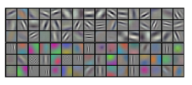
The following figure shows the learnt kernels

Discussion

1. It is notable that our network’s performance degrades if a single convolutional layer is removed. So the depth of the network is important for achieving their results.

2. Their experiments suggest that the results can be improved simply by waiting for faster GPUs and bigger datasets to become available.

Bibliography

<references />