deep Convolutional Neural Networks For LVCSR: Difference between revisions
| Line 31: | Line 31: | ||
= CNN Architecture = | = CNN Architecture = | ||
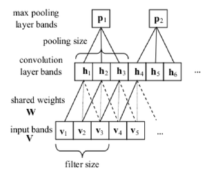
A typical CNN, as shown in Fig 1, consists of a convolutional layer for which the weights are shared across the input space, and a max-poolig layer. | |||
<center> | |||
[[File:Convnets.png |300px | thumb | center |Fig 1. A typical convolutional neural network. ]] | |||
</center> | |||
== Experimental Setup == | == Experimental Setup == | ||
A small 40-hour dataset is used to learn the behaviour of CNNs for speech tasks. The results are reported on EARS dev04f dataset. Features of 40-dimentional log mel-filter bank coeffs are used. The size of the hidden fully connected layer is 1024, and the softmax layer size is 512. For fine-tuning, the learning rate is halved after each iteration for which the objective function doesn't improve sufficiently on a held-out validation set. After 5 times of halving the learning rate, the training stops. | |||
== Number of Convolutional vs. Fully Connected Layers == | == Number of Convolutional vs. Fully Connected Layers == | ||
Revision as of 21:10, 16 November 2015
Introduction
Deep Neural Networks (DNNs) have been explored in the area of speech recognition. They outperformed the-state-of-the-art Gaussian Mixture Models-Hidden Markov Model (GMM-HMM) systems in both small and large speech recognition tasks <ref name=firstDBN> A. Mohamed, G. Dahl, and G. Hinton, “Deep belief networks for phone recognition,” in Proc. NIPS Workshop Deep Learning for Speech Recognition and Related Applications, 2009. </ref> <ref name=tuning_fb_DBN>A. Mohamed, G. Dahl, and G. Hinton, “Acoustic modeling using deep belief networks,” IEEE Trans. Audio Speech Lang. Processing, vol. 20, no. 1, pp. 14–22, Jan. 2012.</ref> <ref name=finetuningDNN> A. Mohamed, D. Yu, and L. Deng, “Investigation of full-sequence training of deep belief networks for speech recognition,” in Proc. Interspeech, 2010, pp. 2846–2849. </ref> <ref name=bing> G. Dahl, D. Yu, L. Deng, and A. Acero, “Context-dependent pretrained deep neural networks for large-vocabulary speech recognition,” IEEE Trans. Audio Speech Lang. Processing, vol. 20, no. 1, pp. 30–42, Jan. 2012. </ref> <ref name=scrf> N. Jaitly, P. Nguyen, A. Senior, and V. Vanhoucke, “An application of pretrained deep neural networks to large vocabulary speech recognition,” submitted for publication. </ref>. Convolutional Neural Networks (CNNs) can model temporal/spacial variations while reduce translation variances. CNNs are attractive in the area of speech recognition for two reasons: first, they are translation invariant which makes them an alternative to various speaker adaptation techniques. Second, spectral representation of the speech has strong local correlations, CNN can naturally capture these type of correlations.
CNNs have been explored in speech recognition <ref name=convDNN> O. Abdel-Hamid, A. Mohamed, H. Jiang, and G. Penn, “Applying convolutional neural networks concepts to hybrid NN-HMM model for speech recognition,” in Proc. ICASSP, 2012, pp. 4277–4280. </ref>, but only one convolutional layer was used. This paper explores using multiple convolutional layers, and the system is tested on one small dataset and two large datasets. The results show that CNNs outperform DNNs in all of these tasks.
CNN Architecture
A typical CNN, as shown in Fig 1, consists of a convolutional layer for which the weights are shared across the input space, and a max-poolig layer.

Experimental Setup
A small 40-hour dataset is used to learn the behaviour of CNNs for speech tasks. The results are reported on EARS dev04f dataset. Features of 40-dimentional log mel-filter bank coeffs are used. The size of the hidden fully connected layer is 1024, and the softmax layer size is 512. For fine-tuning, the learning rate is halved after each iteration for which the objective function doesn't improve sufficiently on a held-out validation set. After 5 times of halving the learning rate, the training stops.
Number of Convolutional vs. Fully Connected Layers
Number of Hidden Units
Optimal Feature Set
Pooling Experiments
Results
Conclusions and Discussions
References
<references />