maximum likelihood estimation of intrinsic dimension

Introduction

In dimensionality reduction (or manifold-learning), the foundation of all methods is the belief that the observed data [math]\displaystyle{ \left\{ \mathbf{x}_{j} \right\} }[/math] are not truly in the high-dimensional [math]\displaystyle{ \mathbb{R}^{D} }[/math]. Rather, there exists a diffemorphic mapping [math]\displaystyle{ \varphi }[/math] such that the data can be efficiently represented in a lower-dimensional space [math]\displaystyle{ \mathbb{R}^{m} }[/math] ([math]\displaystyle{ 0\lt m\lt D }[/math], called intrinsic dimension) by the mapping: [math]\displaystyle{ \mathbf{y}=\varphi(\mathbf{x}), \mathbf{y} \in \mathbb{R}^{m} }[/math]. Most methods (such as PCA, MDS, LLE, ISOMAP, etc.) focus on recover the embedding of high-dimensional data, i.e. [math]\displaystyle{ \left\{ \widehat{\mathbf{y}} \right\} }[/math]. However, there is no consensus on how this intrinsic dimension [math]\displaystyle{ m }[/math] should be determined.

Constructing a reliable estimator of intrinsic dimension will clearly improve the performance of dimensionality reduction methods. Even in supervised learning (such as classification), where the intrinsic dimensionality can be determined by cross-validation. An reliable estimate is still helpful as a guideline for cross-validation to reduce the computational cost.

The problem of estimating the intrinsic dimension is setting up as following: Suppose a set of data points [math]\displaystyle{ \left\{ \mathbf{y}_{j} \right\} }[/math] are sampled i.i.d. from a smooth density [math]\displaystyle{ f(\mathbf{y}) }[/math] on [math]\displaystyle{ \mathbb{R}^{m} }[/math], and mapped into [math]\displaystyle{ \mathbb{R}^{D} }[/math] by a smooth mapping [math]\displaystyle{ \,\psi }[/math], i.e. [math]\displaystyle{ \mathbf{x}_{j}=\psi(\mathbf{y}_{j}),\mathbf{x}_{j} \in \mathbb{R}^{D} }[/math]. The mapping [math]\displaystyle{ \,\psi }[/math] is assumed to be local isometric (not necessarily globally isometric) to ensure that close points in [math]\displaystyle{ \mathbb{R}^{m} }[/math] are mapped closely in [math]\displaystyle{ \mathbb{R}^{D} }[/math]. We only observe [math]\displaystyle{ \left\{ \mathbf{x}_{j} \right\} }[/math]. The low-dimensional data [math]\displaystyle{ \left\{ \mathbf{y}_{j} \right\} }[/math], intrinsic dimension [math]\displaystyle{ m }[/math], the density [math]\displaystyle{ f }[/math] and the mapping [math]\displaystyle{ \psi }[/math] are all unknown. The task is to give an estimator of [math]\displaystyle{ m }[/math] based on above settings.

This paper reviewed several previous works in this topic and proposed a new estimator of intrinsic dimension. The properties of the estimator is discussed and the comparison between this estimator and others is carried out in the numeral experiments.

Previous works

The existing methods for estimating the intrinsic dimensionality can be roughly classified into two types: eigenvalue methods (PCA based), and geometric methods (fractal dimensions).

Eigenvalue methods

PCA can be used to estimate the dimensionality of a globally linear subspace. It assumes in the high-dimensional space, only a linear subspace carries the main variability (main features), and the remaining variabilities are treated as noises. Thus, in global PCA methods, the intrinsic dimension is determined by the number of eigenvalues that are greater than a given threshold.

Global PCA would fail if the underlying manifold is nonlinear. It is intuitive to generalize the idea to local PCA (See Fukunaga and Olsen<ref>Fukunaga, K. and Olsen, D. R. An algorithm for finding intrinsic dimensionality of data. IEEE Trans. on Computers, 1971. </ref> and Bruske and Sommer<ref>Bruske, J. and Sommer, G. Intrinsic dimensionality estimation with optimally topology preserving maps. IEEE Trans. on PAMI, 20(5):572-575, 1998. </ref>). The idea is to choose a set of neighboring points (which is believed to be locally linear) for each points, and apply PCA methods to estimate the dimension of each local region, and the global dimensionality is obtained by summarizing (such as averaging) the local dimensions.

The PCA based methods are intuitive and easy to implement. But the problem is that it is quite sensitive to the choice of local regions (neighborhood size) and thresholds (See Verveer and Duin<ref name="ver">Verveer, P. and Duin, R. An evaluation of intrinsic dimensionality estimators. IEEE Trans. on PAMI, 17(1):81-86, 1995. </ref>).

Geometric methods

The geometric methods try to reveal the intrinsic geometric structure of the observed data. They are usually based on fractal dimension, which is a generalization of topological dimension. The term fractal dimension refers to several different dimension that used to characterize fractals, such as information dimension, capacity dimension, and correlation dimension.

Comparing to eigenvalue methods, geometric methods requires less data points to yeild a reliable estimate (See Lee <ref name="lee">Lee, J. A. Nonlinear Dimensionality Reduction. Springer, New York, Chapter 3, 2007. </ref>). But on the other hand, the geometric methods are computationally more expensive than eigenvalue methods, and they are easier to underestimating the intrinsic dimension for high-dimensional datasets (Verveer and Duin <ref name="ver">Reference</ref>).

Clearly, another potential concern is that the geometric methods still depend on the tuning parameter [math]\displaystyle{ k }[/math] or [math]\displaystyle{ R }[/math].

MLE of intrinsic dimension

The maximum likelihood estimator in general belongs to the geometric methods.

The key assumption for deriving the maximum likelihood estimator of intrinsic dimension is that: For every point [math]\displaystyle{ y\in \mathbb{R}^{m} }[/math], there exists a small sphere [math]\displaystyle{ S_{y}(R) }[/math] of radius [math]\displaystyle{ R }[/math] around [math]\displaystyle{ y }[/math], such that the density [math]\displaystyle{ f(y) \approx const }[/math] within the sphere (i.e. the data points are approximately uniform in each small local region).

For the fixed point [math]\displaystyle{ \,x=\psi(y) }[/math], consider the spatial point process (for more math details about spatial point process, see [1]) [math]\displaystyle{ \left\{ N(t,x), 0 \leq t \leq R \right\} }[/math],

[math]\displaystyle{ N(t,x)=\sum^{n}_{i=1}I(\mathbf{x}_{i} \in S_{x}(t)) }[/math]

which counts observations within distance [math]\displaystyle{ t }[/math] from point [math]\displaystyle{ x }[/math].

With the key assumption and recall the fact that we assume the mapping [math]\displaystyle{ \,\psi }[/math] is local isometric, we can approximate [math]\displaystyle{ \,N(t,x) }[/math] by a poisson process. For the fixed [math]\displaystyle{ x }[/math], ignore the dependence of [math]\displaystyle{ \,N(t,x) }[/math] on [math]\displaystyle{ x }[/math] for now, the rate [math]\displaystyle{ \,\lambda(t) }[/math] of [math]\displaystyle{ \,N(t) }[/math]:

[math]\displaystyle{ \,\lambda(t)=f(y)V(m)mt^{m-1} }[/math]

where [math]\displaystyle{ \,V(m)=\pi^{m/2}[\Gamma(m/2+1)]^{-1} }[/math] is the volume of the unit sphere in [math]\displaystyle{ \mathbb{R}^{m} }[/math]. Letting [math]\displaystyle{ \,\theta=\log f(y) }[/math], we can write the log-likelihood of the observed process [math]\displaystyle{ N(t) }[/math] using the product integration (for details see Snyder<ref>Snyder, D. L. Random Point Process. Wiley, New York, 1975. </ref>):

[math]\displaystyle{ \ell(m,\theta)=\int_{0}^{R}\log \lambda(t)dN(t)-\int_{0}^{R}\lambda(t)dt }[/math]

The MLEs for [math]\displaystyle{ m }[/math] and [math]\displaystyle{ \theta }[/math] exist and are unique with probability goes to 1 as the sample size goes to infinity. The likelihood equations are obtained by taking the partial derivative:

[math]\displaystyle{ \frac{\partial \ell}{\partial \theta}=\int_{0}^{R}dN(t)-\int_{0}^{R}\lambda(t)dt=N(R)-e^{\theta}V(m)R^{m}=0 }[/math] [math]\displaystyle{ \frac{\partial \ell}{\partial m}=\left( \frac{1}{m}+\frac{V^{\prime}(m)}{V(m)} \right)N(R)+\int_{0}^{R}\log t dN(t)-e^{\theta}V(m)R^{m}\left( \log R+\frac{V^{\prime}(m)}{V(m)} \right)=0 }[/math]

Solving the likelihood equations gives the MLE for the intrinsic dimension [math]\displaystyle{ m }[/math]:

[math]\displaystyle{ \widehat{m}_{R}(x)=\left[ \frac{1}{N(R,x)}\sum^{N(R,x)}_{j=1}\log \frac{R}{T_{j}(x)} \right]^{-1} }[/math]

where [math]\displaystyle{ \,T_{j}(x) }[/math] is the Euclidean distance from the fixed point [math]\displaystyle{ x }[/math] to its [math]\displaystyle{ k }[/math]-th nearest neighbor in the sample.

In practice, it can be also expressed in term of the number of neighbors [math]\displaystyle{ k }[/math] rather than the radius of the sphere [math]\displaystyle{ R }[/math]:

[math]\displaystyle{ \widehat{m}_{k}(x)=\left[ \frac{1}{k-1}\sum^{k-1}_{j=1}\log \frac{T_{k}(x)}{T_{j}(x)} \right]^{-1} }[/math]

Remark:

(1). This estimator is a function of a fixed point [math]\displaystyle{ x \in \mathbb{R}^{D} }[/math] and the neighborhood size ([math]\displaystyle{ R }[/math] or [math]\displaystyle{ k }[/math]), so it is an estimate of the local dimensionality at point [math]\displaystyle{ x }[/math].

(2). Like almost all local methods, the choice of neighborhood size clearly affects the performance of the estimator. The general principal of choosing [math]\displaystyle{ k }[/math] (or [math]\displaystyle{ R }[/math]) is to let the sphere to contain sufficiently many data points, and also small enough to satisfy the assumption that [math]\displaystyle{ \,f }[/math] is approximately constant within the sphere.

(3). In the second formula, one may use [math]\displaystyle{ \frac{1}{k-2} }[/math] instead of [math]\displaystyle{ \frac{1}{k-1} }[/math] to get asymptotically unbiased estimator (details will be shown in next subsection).

(4). [math]\displaystyle{ \widehat{\theta} }[/math] can be used to obtain an instant estimate of the entropy of the density [math]\displaystyle{ f }[/math] (See Costa and Hero<ref>Costa, J. and Hero, A. O. Geodesic entropic graphs for dimension and entropy estimation in manifold learning. IEEE Trans. on Signal Processing, 2004. </ref>).

The (global) intrinsic dimension can be estimated by averaging the local dimensions over the whole sample:

[math]\displaystyle{ \widehat{m}_{k}=\frac{1}{n}\sum^{n}_{i=1}\widehat{m}_{k}(\mathbf{x}_{i}) }[/math]

One naive way to make the estimator less sensitive to the choice of neighborhood size [math]\displaystyle{ k }[/math] is to average over a range of different values:

[math]\displaystyle{ \widehat{m}_{(k_{1},k_{2})}=\frac{1}{k_{2}-k_{1}+1}\sum^{k_{2}}_{k=k_{1}}\widehat{m}_{k} }[/math]

Asymptotic behavior of the estimator

The paper also discuss the asymptotic behavior of the estimator. Recall that if we use [math]\displaystyle{ k-2 }[/math] to normalize and use the estimator:

[math]\displaystyle{ \widehat{m}_{k}(x)=\left[ \frac{1}{k-2}\sum^{k-1}_{j=1}\log \frac{T_{k}(x)}{T_{j}(x)} \right]^{-1} }[/math]

Assuming [math]\displaystyle{ m }[/math] is fixed, [math]\displaystyle{ n\rightarrow \infty }[/math], [math]\displaystyle{ k\rightarrow \infty }[/math], and [math]\displaystyle{ k/n\rightarrow 0 }[/math] (or [math]\displaystyle{ R\rightarrow 0 }[/math]). For fixed [math]\displaystyle{ x }[/math], the inhomogeneous process [math]\displaystyle{ \,N(t,x) }[/math] converges weakly to the Poisson process with rate [math]\displaystyle{ \,\lambda(t) }[/math], then [math]\displaystyle{ \,m\log(T_{k}/T_{j}) }[/math] are (asymptotically) distributed as the [math]\displaystyle{ j }[/math]-th order statistic of a sample (with size [math]\displaystyle{ k-1 }[/math]) from standard exponential distribution. To a first order approximation, this gives:

[math]\displaystyle{ U= \frac{1}{m} \sum^{k-1}_{j=1}\log \frac{T_{k}(x)}{T_{j}(x)} \sim Gamma(k-1,1) }[/math]

We can calculate the expectation [math]\displaystyle{ \,E(U^{-1})=1/(k-2) }[/math]. Thus we have:

[math]\displaystyle{ E(\widehat{m}_{k}(x))=d }[/math] [math]\displaystyle{ Var(\widehat{m}_{k}(x))=\frac{m^{2}}{k-3} }[/math]

Remarks:

(1). The estimator of global intrinsic dimension is also asymptotically (in terms of [math]\displaystyle{ n \rightarrow \infty }[/math]) unbiased: [math]\displaystyle{ E(\widehat{m}_{(k_{1},k_{2})})=E(\widehat{m}_{k})=m }[/math]. The variance of [math]\displaystyle{ \widehat{m}_{k} }[/math] is tricky because of the dependence among [math]\displaystyle{ \widehat{m}_{k}(\mathbf{x}_{j}) }[/math]. The paper argues that it can be shown the variance is of order [math]\displaystyle{ n^{-1} }[/math].

(2). The above result is based on a first order approximation, as both [math]\displaystyle{ n,k \rightarrow \infty }[/math], normalizing by [math]\displaystyle{ k-1 }[/math] or [math]\displaystyle{ k-2 }[/math] would both yeild asymptotically unbiased result.

Experiments and comparison

he paper conducts several numerical experiments:

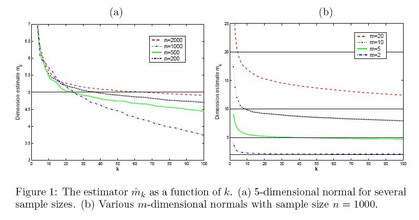
(1). The first experiment is to investigate the properties of the estimator throughout simulations. The estimator [math]\displaystyle{ \widehat{m}_{k} }[/math] is plotted as a function of neighborhood size [math]\displaystyle{ k }[/math] for different sample size (Fig. 1(a)) and different intrinsic dimension (Fig. 1(b)). The result is shown in figure 1.

From figure 1, we can see the effect of [math]\displaystyle{ n,m,k }[/math] on the estimator. Overall, the performance of the MLE is stable and reliable. Certainly the ideal choice of tuning parameter is different for every combination of [math]\displaystyle{ m }[/math] and [math]\displaystyle{ n }[/math], but as can be seen clearly from Fig. 1(a), as the ratio [math]\displaystyle{ k/n }[/math] increases (i.e. the data become sparse and the neighborhood size becomes relatively large), the estimator tends to underestimate the intrinsic dimension.

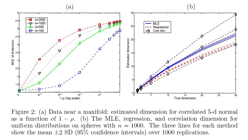
(2). The second experiment is on a 5-dimensional correlated Gaussian distribution wth mean 0 and covariance matrix [math]\displaystyle{ \sigma_{ij}=\rho }[/math] (for [math]\displaystyle{ i\neq j }[/math]), the result is shown in Fig. 2(a). Futhermore, other estimators (correlation dimension, regression dimension) are applied on the same data, and the result is shown in Fig. 2(b).

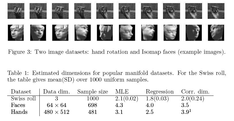
(3). The last experiment is to conduct a comparison between MLE and other estimators on three popular manifold datasets: swiss roll, face image, and hand image. The result is summarized in table 1.

As can be seen, for swiss roll data (small dimension, large sample size), the MLE provide the best result among three. But as dimension increases (and sample size decreases), the MLE does not work so well.

Discussion

(1). Under certain assumptions the MLE of intrinsic dimension has nice asymptotic properties, and the simulated data and some real dataset also show the performance of MLE is reliable (comparing to other geometric method).

(2). The MLE does NOT work so well on high-dimensional data (suffer from a negative bias), because the key assumption (sufficiently many observations within a small sphere) is always violated in real high-dimensional space (the curse of dimensionality), so it is almost impossible to find a ideal neighborhood size. The effect is similar to what has been shown in Fig. 1(a).

(3). For some datasets, such as points in a unit cube, there is also the issue of edge effects, which will also cause the negative bias. One can potentially reduce the bias by removing the edge points by some criterion. However, the author claims that the edge effects are small compared to the sample size problem.

(4). The paper uses Poisson distribution assumption and in order to use MLE, they assume that all the sample points share the same parameter. However, the density around each sample points is different for real data. This might affect the estimation of dimensionality.

References

<references />