sparse PCA: Difference between revisions
Mirzazadeh (talk | contribs) |
Mirzazadeh (talk | contribs) |
||
| Line 100: | Line 100: | ||
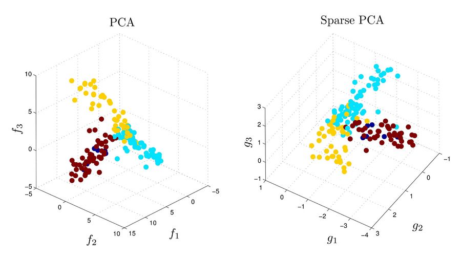
three components. For the PCA, each principal component is a combination of all 500 variables (corresponding to 500 genes) while in sparse PCA each involves variables corresponding to at most 6 genes. | three components. For the PCA, each principal component is a combination of all 500 variables (corresponding to 500 genes) while in sparse PCA each involves variables corresponding to at most 6 genes. | ||
[[Image:Spca-g.jpg|thumb|900px|center|Distribution of gene expression data in the PCA vs. Sparse PCA. The point colors are based on an pre-computed independent clustering.]] | [[Image:Spca-g.jpg|thumb|900px|center|Distribution of gene expression data in the PCA vs. Sparse PCA. The point colors are based on an pre-computed independent clustering.]] | ||
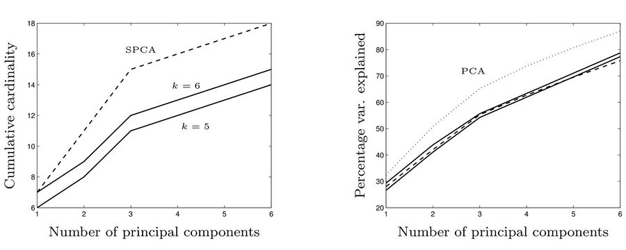
In the next figure, the left diagram compares the number of non-zero elements in principal components in three methods: SPCA, the method we explaind with <math>k=5</math>, and the method we explaind with <math>k=6</math>. In the right diagram, the percentage of total variance explained by the first six principle components resulted from PCA, SPCA (dashed) and the method we explained with <math>k=5</math> and <math>k=6</math> (solid lines). | |||
[[Image:Spca-a.jpg|thumb|900px|center|Distribution of gene expression data in the PCA vs. Sparse PCA. The point colors are based on an pre-computed independent clustering.]] | |||
Revision as of 17:30, 28 June 2009
Introduction
Given [math]\displaystyle{ n }[/math] observations on [math]\displaystyle{ d }[/math] variables (or in other words [math]\displaystyle{ n }[/math] [math]\displaystyle{ d }[/math]-dimensional data points), in PCA the goal is to find directions in the data set space that correspond to the directions with biggest variance in the input data. In the practice each of the [math]\displaystyle{ d }[/math] variables has its own special meaning and it may be desirable to come up with some directions, as principal components, each of which is a combination of just a few of these variables. This makes the directions more interpretable and meaningful. But this is not something that usually happens in the oridinal result of PCA method. Each of resulting directions from PCA in most cases is rather a linear combination of all variable with no zero coefficients.
The address the above concern we add a sparsity constraint to the PCA problem, which makes the PCA problem much harder to solve. That's because we have just added a combinatorial constraint to out optimization problem. This paper is about how to find directions in the data space with maximum variance that have a limited number of non-zero elements.
Problem Formulation
Given the covariance matrix [math]\displaystyle{ A }[/math], the problem can be written as:
|
[math]\displaystyle{ \begin{array}{ll} \textrm{maximize}& x^TAx\\ \textrm{subject\ to}& ||x||_2=1\\ &\textbf{Card}(x)\leq k \end{array} }[/math] | (1) |
Defining [math]\displaystyle{ X=x^Tx }[/math], the above formula can be rewritten as
|
[math]\displaystyle{ \begin{array}{ll} \textrm{maximize}& \textbf{Tr}(AX)\\ \textrm{subject\ to}&\textbf{Tr}(X)=1\\ &\textbf{Card}(x)\leq k^2\\ &X\succeq 0, \textbf{Rank}(X)=1\\ \end{array} }[/math] | (2) |
The conditions [math]\displaystyle{ X\succeq 0 }[/math] and [math]\displaystyle{ \textbf{Rank}(X)=1 }[/math] in formula 2 guarantees that [math]\displaystyle{ X }[/math] can be written as [math]\displaystyle{ x^Tx }[/math], for some [math]\displaystyle{ x }[/math]. But this formulation should be relaxed before it can be solved efficiently, because the constraintS [math]\displaystyle{ \textbf{Card}(x)\leq k^2 }[/math] and [math]\displaystyle{ \textbf{Rank}(X)=1 }[/math] are not convex. So we replace the cardinality constraint with a weaker one: [math]\displaystyle{ \textbf{1}^T|X|\textbf 1\leq k }[/math]. We also drop the rank constraint. So we get:
|
[math]\displaystyle{ \begin{array}{ll} \textrm{maximize}& \textbf{Tr}(AX)\\ \textrm{subject\ to}&\textbf{Tr}(X)=1\\ &\textbf{1}^T|X|\textbf 1\leq k\\ &X\succeq 0\\ \end{array} }[/math] |
We then change the modified cardinality constraint to a penalty term in the goal function with some positive factor [math]\displaystyle{ \rho }[/math]. So we get a semidefinite form of the problem:
|
[math]\displaystyle{ \begin{array}{ll} \textrm{maximize}& \textbf{Tr}(AX)-\rho\textbf{1}^T|X|\textbf 1\\ \textrm{subject\ to}&\textbf{Tr}(X)=1\\ &X\succeq 0\\ \end{array} }[/math] | (3) |
The goal function can be rewritten as [math]\displaystyle{ \textbf{Tr}(AX)-\rho\textbf{1}^T|X|\textbf 1=\min_{|U_{ij}|\leq\rho}\textbf{Tr}((A+U)X) }[/math]. So the problem (3) is equivalent to:
|
[math]\displaystyle{ \begin{array}{ll} \textrm{maximize}& \min_{|U_{ij}|\leq\rho}\textbf{Tr}(X(A+U)\\ \textrm{subject\ to}&\textbf{Tr}(X)=1\\ &X\succeq 0\\ \end{array} }[/math] | (4) |
or equivalently:
|
[math]\displaystyle{ \begin{array}{lll} \textrm{minimize}& \lambda^{\max}(A+U))\\ \textrm{subject\ to}&|U_{ij}|\leq\rho,&i,j=1\cdots,n\\ \end{array} }[/math] | (5) |
The problem as described in formulation (5) can be seen as computing a robust version of maximum eigenvalue: it is the least possible value of maximum eigenvalue, given that each element can be changed by at most noise value [math]\displaystyle{ \rho }[/math].
The Algorithm
The Main Loop
The algorithm should iteratively create the semidefinite program (4) and solve it to obtain the next most important sparse principle component. At each iteration, if [math]\displaystyle{ X }[/math] is the optimal solution of the optimization problem, we first need to obtain the solution [math]\displaystyle{ x }[/math] of the corresponding problem of form (1). That will be straightforward if [math]\displaystyle{ X }[/math] is of rank 1, but since we have dropped the rank constraint, this may not be true and in those cases we need to obtain the dominant eigenvalue of [math]\displaystyle{ X }[/math] by methods that are known in the literature. After obtaining a (hopefully) sparse vector [math]\displaystyle{ x }[/math] we replace the matrix [math]\displaystyle{ A }[/math] with [math]\displaystyle{ A-(x_1^TAx_1)x_1x_1^T }[/math] and repeat the above steps to obtain next sparse component values.
The question then is when to stop. Two approaches are proposed. First is that at each iteration [math]\displaystyle{ i }[/math], for all [math]\displaystyle{ i\lt j }[/math], we include the constraint [math]\displaystyle{ x_i^TXx_i=0 }[/math] to make sure each principal component we compute is orthogonal to the previous ones. Then the procedure stops after [math]\displaystyle{ n }[/math] steps automatically (there will be no solution to the [math]\displaystyle{ n+1 }[/math]'th problem). The other way is stop as soon as all members of [math]\displaystyle{ A }[/math] get less than [math]\displaystyle{ \rho }[/math], because at that point elements of [math]\displaystyle{ A }[/math] will be less than the noise value [math]\displaystyle{ \rho }[/math].
Solving the Semidefinite Problem
The cardinality constraint in the formulation (or its corresponding term in the penalized form) introduces a quadratic number of terms in the problem. This makes it practically impossible to use interior-point method to solve the problem for large values of the input dimension. So we need to use other existing methods for solving the problem, but then, there will be a matter of speed. Denoting the required accuracy by [math]\displaystyle{ \epsilon }[/math], we can expect an interior-point-based program to converge after [math]\displaystyle{ \textstyle O(F(n)\log\frac1{\epsilon}) }[/math] iterations, for some function [math]\displaystyle{ F }[/math] of input size [math]\displaystyle{ n }[/math]. Here we will manage to solve the problem using [math]\displaystyle{ \textstyle O(\frac{F(n)}{\epsilon}) }[/math] iterations using a first-order scheme, for some function [math]\displaystyle{ F }[/math] of input size.
First-order method can solve a problem after [math]\displaystyle{ \textstyle O(\frac1{\epsilon}) }[/math] iterations, for some function [math]\displaystyle{ F }[/math] of input size, if the problem satisfy a smoothness constraint. But in our case, [math]\displaystyle{ X\succeq 0 }[/math] is not smooth and as a result, an application of first-order method to the our problem will result in an algorithm stopping after [math]\displaystyle{ \textstyle O(\frac1{\epsilon^2}) }[/math] iterations, for some function [math]\displaystyle{ F }[/math] of input size, which is too slow. To address this problem, we consider the formulation (5) and then we define a smooth approximation of the function [math]\displaystyle{ \lambda^{\max} }[/math].
To come up with a smooth approximation of our goal function, we define [math]\displaystyle{ f_{\mu}(X)=\mu\log\textbf{Tr}(e^{\frac X\mu}) }[/math]. Then, one can verify that [math]\displaystyle{ \lambda^{\max}(X)\leq f_\mu(X)\leq\lambda^{\max}(X)+\mu\log n }[/math] and so, for [math]\displaystyle{ \textstyle\mu=\frac{\epsilon}{\log n} }[/math], [math]\displaystyle{ f_{\mu} }[/math] is a smooth approximation of [math]\displaystyle{ \lambda^{\max} }[/math] with an additive error of [math]\displaystyle{ \epsilon }[/math]. This way we obtain a scheme for solving the program in [math]\displaystyle{ \textstyle\frac d{\epsilon}\sqrt{\log d} }[/math] iterations, each taking [math]\displaystyle{ O(d^3) }[/math] time.
Experimental Results
Each point in figures below corresponds to an experiment on 500 genes. The points are pre-clustered to 4 clusters based some prior knowledge. The top three principal components are computed using each of PCA and Sparse PCA methods, and the points are plotted in the bases defined by these three components. For the PCA, each principal component is a combination of all 500 variables (corresponding to 500 genes) while in sparse PCA each involves variables corresponding to at most 6 genes.

In the next figure, the left diagram compares the number of non-zero elements in principal components in three methods: SPCA, the method we explaind with [math]\displaystyle{ k=5 }[/math], and the method we explaind with [math]\displaystyle{ k=6 }[/math]. In the right diagram, the percentage of total variance explained by the first six principle components resulted from PCA, SPCA (dashed) and the method we explained with [math]\displaystyle{ k=5 }[/math] and [math]\displaystyle{ k=6 }[/math] (solid lines).
