stat340s13

Introduction, Class 1 - Tuesday, May 7

{{

 Template:namespace detect

| type = style | image = | imageright = | style = | textstyle = | text = This article may require cleanup to meet Wikicoursenote's quality standards. The specific problem is: use math environment and LaTex notations for formulas. For example instead of y=1-e^(-λx) write [math]\displaystyle{ y=1-e^{-\lambda x} }[/math]. Please improve this article if you can. | small = | smallimage = | smallimageright = | smalltext = }}

Course Instructor: Ali Ghodsi

Lecture:
001: TTh 8:30-9:50 MC1085
002: TTh 1:00-2:20 DC1351
Tutorial:
2:30-3:20 Mon M3 1006

Midterm

Monday June 17 2013 from 2:30-3:30

TA(s):

Lu Cheng Monday 3:30-5:30 pm M3 3108 space 2
Han ShengSun Tuesday 4-6 pm M3 3108 space 2
Yizhou Fang Wednesday 1-3 pm M3 3108 space 1
Huan Cheng Thursday 3-5 pm M3 3111 space 1
Wu Lin Friday 11am - 1pm M3 3108 space 1

Four Fundamental Problems

1. Classification: Given an input object X, we have a function which will take in this input X and identify which 'class (Y)' it belongs to (Discrete Case)
(For example, an image of a fruit can be classified, through some sort of algorithm to be a picture of either an apple or an orange.)
2. Regression: Same as classification but in the continuous case except y is discrete
3. Clustering: Use common features of objects in same class or group to form clusters.(in this case, x is given, y is unknown)
4. Dimensionality Reduction (aka Feature extraction, Manifold learning)

Applications

Most useful when structure of the task is not well understood but can be characterized by a dataset with strong statistical regularit y
Examples:

• Computer Vision, Computer Graphics, Finance (fraud detection), Machine Learning
  
• Search and recommendation (eg. Google, Amazon)
  
• Automatic speech recognition, speaker verification
  
• Text parsing
  
• Face identification
  
• Tracking objects in video
  
• Financial prediction(e.g. credit cards)
  
• Fraud detection
  
• Medical diagnosis
  

Course Information

Prerequisite: (One of CS 116, 126/124, 134, 136, 138, 145, SYDE 221/322) and (STAT 230 with a grade of at least 60% or STAT 240) and (STAT 231 or 241)

Antirequisite: CM 361/STAT 341, CS 437, 457

General Information

• No required textbook
• Recommended: "Simulation" by Sheldon M. Ross
• Computing parts of the course will be done in Matlab, but prior knowledge of Matlab is not essential (will have a tutorial on it)
• First midterm will be held on Monday, June 17 from 2:30 to 3:30
• Announcements and assignments will be posted on Learn.
• Other course material on: http://wikicoursenote.com/wiki/
• Log on to both Learn and wikicoursenote frequently.
• Email all questions and concerns to UWStat340@gmail.com. Do not use your personal email address!

Wikicourse note (10% of final mark): When applying an account in the wikicourse note, please use the quest account as your login name while the uwaterloo email as the registered email. This is important as the quest id will use to identify the students who make the contributions. Example:
User: questid
Email: questid@uwaterloo.ca
After the student has made the account request, do wait for several hours before students can login into the account using the passwords stated in the email. During the first login, students will be ask to create a new password for their account.

As a technical/editorial contributor: Make contributions within 1 week and do not copy the notes on the blackboard.

Must do both All contributions are now considered general contributions you must contribute to 50% of lectures for full marks

• A general contribution can be correctional (fixing mistakes) or technical (expanding content, adding examples, etc) but at least half of your contributions should be technical for full marks

Do not submit copyrighted work without permission, cite original sources. Each time you make a contribution, check mark the table. Marks are calculated on honour system, although there will be random verifications. If you are caught claiming to contribute but didn't, you will lose marks.

Wikicoursenote contribution form : [1]

- you can submit your contributions in multiple times.
- you will be able to edit the response right after submitting
- send email to make changes to an old response : uwstat340@gmail.com

Tentative Topics

- Random variable and stochastic process generation
- Discrete-Event Systems
- Variance reduction
- Markov Chain Monte carlo

Tentative Marking Scheme

Item	Value
Assignments (~6)	30%
WikiCourseNote	10%
Midterm	20%
Final	40%

To pass the course, you need to pass the final exam

Sampling (Generating random numbers), Class 2 - Thursday, May 9

Introduction

There are camps debating about sampling. Some people believe that activities such as rolling a dice and flipping a coin are not truly random but are deterministic – the result can be reliably calculated using things such as physics and math.

A computer cannot generate truly random numbers since computers can only run algorithms, which are deterministic in nature. They can, however, generate Pseudo Random Numbers; numbers that seem random but are actually deterministic. Although the pseudo random numbers are deterministic, these numbers have a sequence of value and all of them have the appearances of being independent uniform random variables.

Mod

Let [math]\displaystyle{ n \in \N }[/math] and [math]\displaystyle{ m \in \N^+ }[/math], then by Divisioin Algorithm, [math]\displaystyle{ \exists! q, \, r \in \N \;\text{with}\; 0\leq r \lt m, \; \text{s.t.}\; n = mq+r }[/math], where [math]\displaystyle{ q }[/math] is called the quotient and [math]\displaystyle{ r }[/math] the remainder. Hence we can define a binary function [math]\displaystyle{ \mod : \N \times \N^+ \rightarrow \N }[/math] given by [math]\displaystyle{ r:=n \mod m }[/math].
Note: [math]\displaystyle{ \mod }[/math] here is different from the modulo congruence relation in [math]\displaystyle{ \Z_m }[/math], which is an equivalence relation instead of a function.

Multiplicative Congruential Algorithm

This is a simple algorithm used to generate uniform pseudo random numbers. It is also referred to as the Linear Congruential Method or Mixed Congruential Method. We define the Linear Congruential Method to be [math]\displaystyle{ x_{k+1}=(ax_k + b) \mod m }[/math], where [math]\displaystyle{ x_k, a, b, m \in \N, \;\text{with}\; a, m \gt 0 }[/math]. Given a "seed" [math]\displaystyle{ x_0 \in \N }[/math], we can obtain values for [math]\displaystyle{ x_1, \, x_2, \, \cdots, x_n }[/math] inductively. The Multiplicative Congruential Method may also refer to the special case where [math]\displaystyle{ b=0 }[/math].

Algorithm 1
x_k+1 = x_k mod m

Example
Let x₀ = 10, m = 3
Step 1: 1 = 10 mod 3
Step 2: 1 = 1 mod 3
Step 3: 1 = 1 mod 3
... This method generates a sequence of identical integers, hence we need a better algorithm.

Algorithm 2 (Multiplicative Congruential Algorithm)
x_k+1 = (a*x_k+b) mod m

Example
Let a = 2, b = 1, m = 3, x₀ = 10
Step 1: 0 = (2*10+1) mod 3
Step 2: 1 = (2*0+1) mod 3
Step 3: 0 = (2*1+1) mod 3
This method generates a sequence with a repeating cycle of two integers.

(if people choose numbers properly, they could get a random sequence of numbers. However, how do we find the value of a,b, and m? At the very least m should be a very large, preferably prime number. The larger m is, the more possibility people get a random sequence of numbers. This is easier to solve in Matlab. In Matlab, rand() generates random numbers those are uniformly distributed in the interval (0,1)). Matlab uses a=7⁵, b=0, m=2³¹-1

MatLab Instruction for Multiplicative Congruential Algorithm:
Before you start:

>>clear all
>>close all

>>a=17
>>b=3
>>m=31
>>x=5
>>mod(a*x+b,m)
ans=26
>>x=mod(a*x+b,m)

(Note:
1. Keep repeating this command over and over again and you will seem to get random numbers – this is how the command rand works in a computer.
2. There is a function called RAND to generate a number between 0 and 1. 3. If we would like to generate 1000 and more numbers, we could use a for loop)

>>a=13
>>b=0
>>m=31
>>x(1)=1
>>for ii=2:1000
x(ii)=mod(a*x(ii-1)+b,m);
end
>>size(x)
ans=1    1000
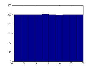
>>hist(x)

(Note: The semicolon after the x(ii)=mod(a*x(ii-1)+b,m) ensures that Matlab will not show the entire vector of x. It will instead calculate it internally and you will be able to work with it. Adding the semicolon to the end of this line reduces the run time significantly.)

This algorithm involves three integer parameters a, b, and m and an initial value, x₀ called seed. A sequence of numbers is defined by x_k+1 = a*x_k + b mod m. Mod m means take the remainder after division by m.

Note: For some bad a and b, the histogram may not be uniformly distributed.

Example: a=13, b=0, m=31
The first 30 numbers in the sequence are a permutation of integers for 1 to 30 and then the sequence repeats itself so it is important to choose m large. Values are between 0 and m-1. If the values are normalized by dividing by m-1, then the result is numbers uniformly distributed in the interval [0,1]. There is only a finite number of values (30 possible values in this case). In Matlab, you can use function "hist(x)" to see if it is uniformly distributed.

If x₀ =1, then

[math]\displaystyle{ x_{k+1} = 13x_{k}\mod{31} }[/math]

So,

[math]\displaystyle{ \begin{align} x_{0} &{}= 1 \end{align} }[/math]

[math]\displaystyle{ \begin{align} x_{1} &{}= 13 \times 1 + 0\mod{31} = 13 \\ \end{align} }[/math]

[math]\displaystyle{ \begin{align} x_{2} &{}= 13 \times 13 + 0 \mod{31} = 14 \\ \end{align} }[/math]

[math]\displaystyle{ \begin{align} x_{3} &{}= 13 \times 14 + 0 \mod{31} =27 \\ \end{align} }[/math]

etc.

For example, with a = 3, b = 2, m = 4, x₀ = 1, we have:

[math]\displaystyle{ x_{k+1} = (3x_{k} + 2)\mod{4} }[/math]

So,

[math]\displaystyle{ \begin{align} x_{0} &{}= 1 \end{align} }[/math]

[math]\displaystyle{ \begin{align} x_{1} &{}= 3 \times 1 + 2 \mod{4} = 1 \\ \end{align} }[/math]

[math]\displaystyle{ \begin{align} x_{2} &{}= 3 \times 1 + 2 \mod{4} = 1 \\ \end{align} }[/math]

etc.

---

FAQ:

1.Why in the example above is 1 to 30 not 0 to 30?
2.Will the number 31 ever appear?Is there a probability that a number never appears?

---

Examples:[From Textbook]
If x₀=3 and x_n=(5x_n-1+7)mod 200, find x₁,...,x₁₀.
Solution:
x₁= (15+7) mod 200= 22
x₂= 117 mod 200= 117
x₃= 592 mod 200 = 192
x₄= 2967 mod 200= 167
x₅= 14842 mod 200= 42
x₆= 74217 mod 200 = 17
x₇= 371092 mod 200= 92
x₈= 1855467 mod 200= 67
x₉= 9277342 mod 200 = 142
x₁₀= 46386717 mod 200 = 117

Comments:
Typically, it is good to choose m such that m is large, and m is prime. Careful selection of parameters 'a' and 'b' also helps generate relatively "random" output values, where it is harder to identify patterns. For example, when we used a non prime number such as 40 for m, our results were not satisfactory in producing an output resembling a uniform distribution.

The computed values are between 0 and m-1. If the values are normalized by dividing by m-1, their result is numbers uniformly distributed on the interval [0,1] (similar to computing from uniform distribution).

From the example shown above, we can see to create a good random number sequence generator, we need to select a large m. As the x_n value is dependent on the (5x_n-1+7)value, such that the value it can be is between 0 to m after that a value will be repeated; and once this happens the whole sequence will began to repeat. Thus, if we want to create large group of random number, it is better to have large m such that the random value generated will not be repeated after several recursion.
Example:
For x_n = (2x_n-1+1) mod 3 where x₀=2, x₁ = 5 mod 3 = 2
Notice that, with the small value m, the random number generated repeated itself is faster than when the value is large enough.

For many years the “rand” function in Matlab used this algorithm with these parameters A=7⁵=16807, b=0, m=2³¹ -1=2147483647 – recommended in a 1988 paper, "Random Number Generators: Good Ones Are Hard To Find" by Stephen K. Park and Keith W. Miller (Important part is that m should be large)

There has been a research about how to choose uniform sequence. Many programs give you the chance to choose the seed. Sometimes the first number is chosen by CPU.

Moreover, it is fact that not all variables are uniform. Some has normal distribution, or exponential distribution, or binomial distribution as well.

Inverse Transform Method

This method is useful for generating types of distribution other than uniform distribution, such as exponential distribution and normal distribution. However, to use this method in generating pseudorandom numbers, the probability distribution consumed must be a cdf such that it is continuous for the F^-1 always exists. Exponential distribution has the property that generated numbers are frequently close to 0. Normal distribution has the property that generated numbers are frequently close to its mean.

Theorem:
Take U ~ U[0,1] and let [math]\displaystyle{ x=F^{-1}(U) }[/math] Then x has distribution function F(•)
Where [math]\displaystyle{ F(x) = P(X }[/math] ≤ [math]\displaystyle{ x) }[/math] is the CDF and;
[math]\displaystyle{ F^{-1}(U) }[/math]denotes the inverse function of F(•) Or that [math]\displaystyle{ F(x)=U }[/math] [math]\displaystyle{ \Rightarrow }[/math] [math]\displaystyle{ x=F^{-1}(U) }[/math]

Proof of the theorem:
[math]\displaystyle{ F(x) = P(X }[/math] ≤ [math]\displaystyle{ x) }[/math]
[math]\displaystyle{ F(x) = P(F^{-1}(U) }[/math] ≤ [math]\displaystyle{ x) }[/math]
[math]\displaystyle{ F(x) = P(F(F^{-1}(U)) }[/math] ≤ [math]\displaystyle{ F(x)) }[/math]  ::"Applying F, which is monotonic, to both sides"
[math]\displaystyle{ F(x) = P(U }[/math] ≤ [math]\displaystyle{ F(x)) }[/math]
[math]\displaystyle{ F(x) = F(x) }[/math]  ::"Because [math]\displaystyle{ Pr(U }[/math] ≤ [math]\displaystyle{ y)=y }[/math],since U is uniform on the unit interval"

F(^.) is a monotonic function, which is a function that strictly increasing or decreasing.

Example: [math]\displaystyle{ f(x) = \lambda e^{-\lambda x} }[/math]
[math]\displaystyle{ F(x)= \int_0^x f(x) dx }[/math]
[math]\displaystyle{ = \int_0^x \lambda e ^{-\lambda x}\ dx }[/math]
[math]\displaystyle{ = \frac{\lambda}{-\lambda}\, e^{-\lambda x}\, | \underset{0}{x} }[/math]
[math]\displaystyle{ = -e^{\lambda x} + e^0 }[/math]
[math]\displaystyle{ =1 - e^{- \lambda x} }[/math]
[math]\displaystyle{ y=1-e^{- \lambda x} }[/math]
[math]\displaystyle{ 1-y=e^{- \lambda x} }[/math]
[math]\displaystyle{ x=-ln(1-y)/{\lambda} }[/math]
[math]\displaystyle{ y=-ln(1-x)/{\lambda} }[/math]
[math]\displaystyle{ F^{-1}(x)=-ln(1-x)/{\lambda} }[/math]

Step 1: Draw U ~U[0,1];
Step 2: [math]\displaystyle{ x=\frac{-ln(1-U)}{\lambda} }[/math]

Example: [math]\displaystyle{ X= a + (b-a), }[/math] U is uniform on [a, b]
[math]\displaystyle{ x=\frac{-ln(U)}{\lambda} }[/math] is exponential with parameter [math]\displaystyle{ {\lambda} }[/math]

Example 2: Given a CDF of X: [math]\displaystyle{ F(x) = x^5 }[/math], transform U~U[0,1].
Sol: Let [math]\displaystyle{ y=x^5 }[/math], solve for x: [math]\displaystyle{ x=y^{1/5} }[/math]. Therefore, [math]\displaystyle{ F^{-1} (x) = x^{1/5} }[/math]
Hence, to obtain a value of x from F(x), we first set u as an uniform distribution, then obtain the inverse function of F(x), and set [math]\displaystyle{ x= u^{1/5} }[/math]

In Matlab, you can use functions: "who" to see what variables you have defined "clear all" to clear all variables you have defined "close all" to close all figures

MatLab for Inverse Transform Method:

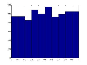
>>u=rand(1,1000)
>>hist(u)       #will generate a fairly uniform diagram

#let λ=2 in this example; however, you can make another value for λ
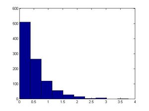
>>x=(-log(1-u))/2;
>>size(x)       #1000 in size 
>>figure
>>hist(x)       #exponential 

Limitations:
1. This method is flawed since not all functions are invertible nor monotonic.
2. It may be impractical since some CDF's and/or integrals are not easy to compute.

Probability Distribution Function Tool in MATLAB

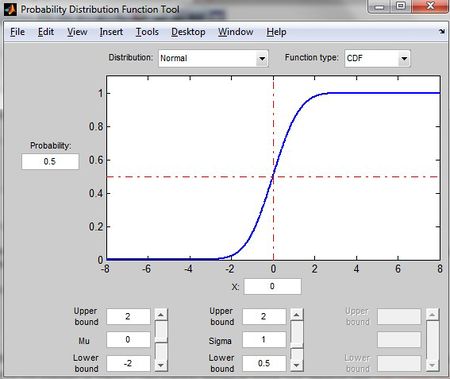
>>disttool         #shows different distributions

This command allows users to explore the effect of changes of parameters on the plot of either a CDF or PDF.

(Generating random numbers continue) Class 3 - Tuesday, May 14

---

Discrete Case:
The method used for continuous case can also be applied to the discrete case:
We want to generate a discrete random variable x, that has probability mass function: In general in the discrete case, we have [math]\displaystyle{ x_0, \dots , x_n }[/math] where:

[math]\displaystyle{ \begin{align}P(X = x_i) &{}= p_i \end{align} }[/math]

[math]\displaystyle{ x_0 \leq x_1 \leq x_2 \dots \leq x_n }[/math]

[math]\displaystyle{ \sum p_i = 1 }[/math]

1: Draw [math]\displaystyle{ U~ \sim~ Unif [0,1] }[/math]
2. [math]\displaystyle{ X=x_i, }[/math] if [math]\displaystyle{ F(x_{i-1})\lt U\lt F(x_i) }[/math]
Example (from class):

Suppose we have the following discrete distribution:

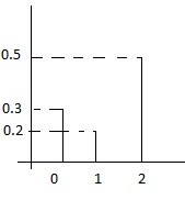
[math]\displaystyle{ \begin{align} P(X = 0) &{}= 0.3 \\ P(X = 1) &{}= 0.2 \\ P(X = 2) &{}= 0.5 \end{align} }[/math]

The cumulative density function (cdf) for this distribution is then:

[math]\displaystyle{ F(x) = \begin{cases} 0, & \text{if } x \lt 0 \\ 0.3, & \text{if } 0 \leq x \lt 1 \\ 0.5, & \text{if } 1 \leq x \lt 2 \\ 1, & \text{if } 2 \leq x \end{cases} }[/math]

Then we can generate numbers from this distribution like this, given [math]\displaystyle{ U \sim~ Unif[0, 1] }[/math]:

[math]\displaystyle{ x = \begin{cases} 0, & \text{if } U\leq 0.3 \\ 1, & \text{if } 0.3 \lt U \leq 0.5 \\ 2, & \text{if } 0.5 \lt U\leq 1 \end{cases} }[/math]

Example: Generating a Bernoulli random variable

[math]\displaystyle{ \begin{align} P(X = 1) = p, P(X = 0) = 1 - p\end{align} }[/math]

[math]\displaystyle{ F(x) = \begin{cases} 1-p, & \text{if } x \lt 1 \\ p, & \text{if } 1 \leq x \end{cases} }[/math]

1. Draw [math]\displaystyle{ U~ \sim~ Unif [0,1] }[/math]
2. [math]\displaystyle{ X = \begin{cases} 1, & \text{if } U\leq p \\ p, & \text{if } U \gt p \end{cases} }[/math]

Note: Unlike the continuous case, the discrete inverse-transform method can always be used for any discrete distribution (but it may not be the most efficient approach)

Review for last class
Inverse Transform Method
1. Draw U~U(0,1)
2. X = F^-1(U)

Proof
P(X<=x)
= P(F^-1(U)<=x)
= P(F(F^-1(U))<=F(x))
= P(U<=F(x))
=F(x)
This is the c.d.f. of X

Remainder:
This is only for uniform distribution [math]\displaystyle{ U~ \sim~ Unif [0,1] }[/math]
P(U<=1)=1
P(U<=0.5)=0.5

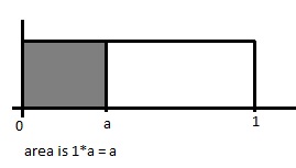[math]\displaystyle{ P(U\lt =a)=a }[/math]

Example in class
Just like flipping a coin, we have 50% chance to get head and 50% chance to get tail.
[math]\displaystyle{ U~ \sim~ Unif [0,1] }[/math]

[math]\displaystyle{ \begin{align} P(X = 0) &{}= 0.5\\ P(X = 1) &{}= 0.5\\ \end{align} }[/math]

• Code
  

 [math]\displaystyle{ \text{if } U\leq 0.5  }[/math]

    [math]\displaystyle{ X = 0 }[/math] 

 [math]\displaystyle{ \text{else if }0.5 \leq U\leq 1  }[/math]

    [math]\displaystyle{ X = 1 }[/math] 

 [math]\displaystyle{  \text{end }  }[/math]

Example in class:

p(x=0)=0.3
p(x=1)=0.2
p(x=2)=0.5
F(x)=0 If x<0
F(x)=0.3 if 0<=x<1
F(x)=0.5 if 1<x<2
F(x)=1 x>=2

x=0 if u<0.3
x=1 if 0.3<=u<0.5
x=2 if x>=0.5

Matlab code in class

Use Editor window to edit the code
close all
clear all
for ii=1:1000


   u=rand;

   if u<0.3

      x(ii)=0;

   elseif u<0.5

      x(ii)=1;

   else

      x(ii)=2;

   end

end

(F5-save and run)

>>size(x)
>>hist(x)


Acception-Rejection Method

Although the inverse transformation method does allow us to change our uniform distribution, it has two limits;

1. Not all functions have an inverse
2. For some distributions, such as Gaussian, it is far too difficult to find the inverse

To generate random samples for these functions, we must use different methods, such as the Acception Rejection Method.

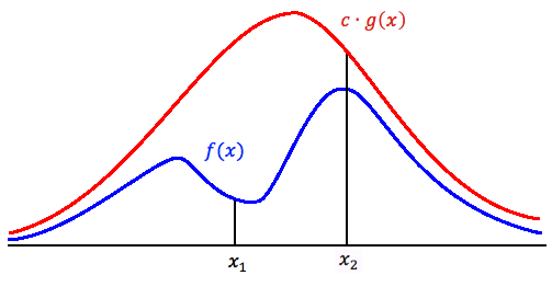
Note that g(x) can generate more than what we need. It can also generate less than what we need. But for c*g(x) >= f(x), in any region, it can generate at least equal to what we need.

value around x1 will be sampled more often under cg(x) than under f(x).

around x2:number of sample that are drawn and the number we need are much closer.

Procedure

1. Draw y~g
2. Draw u~u(0,1)
3. If [math]\displaystyle{ u\lt =(f(y)/cg(y)) }[/math] (which is P(accepted|y)) then x=y, else return to 1

[math]\displaystyle{ P(y|accepted)=f(y) }[/math] [math]\displaystyle{ P(y|accepted)=(P(accepted|y)*P(y))/P(accepted) }[/math]
Recall: [math]\displaystyle{ P(a|b)=P(a,b)/P(b) }[/math], or [math]\displaystyle{ P(a|b)=P(b|a)*P(a)/P(b) }[/math]
as we know, [math]\displaystyle{ P(y)=g(y) }[/math]
[math]\displaystyle{ P(accepted|y)=f(y)/(c*g(y)) }[/math]
[math]\displaystyle{ P(accepted)=\int_y\ P(accepted|y)*P(y)= \int_y\ f(s)/(c*g(s))*g(x) ds=1/c \int_y\ f(s) ds\lt br /\gt =1/c }[/math]
Therefore, [math]\displaystyle{ P(y|accepted)=f(y)/(c*g(y))/1/c=f(y)/(c*g(y))/1/c=f(y) }[/math]

Acceptance-Rejection Method Example 1 (discrete case) We wish to generate X~Bi(2,0.5), assuming that we cannot generate this directly. We use a discrete distribution DU[0,2] to approximate this. f(x)=Pr(X=x)=2Cx*(0.5)^2 x 0 1 2 f(x) 1/4 1/2 1/4 g(x) 1/3 1/3 1/3 c=f(x)/g(x) 3/4 3/2 3/4 f(x)/(c*g(x)) 1/2 1 1/2

Since we need c>=f(x)/g(x) We need c=3/2

Therefore, the algorithm is: 1. Generate u,v~U(0,1) 2. Set y=floor(3*u) (This is using uniform distribution to generate DU[0,2] 3. If (y=0) and (v<1/2), output=0 If (y=2) and (v<1/2), output=2 Else if y=1, output=1

An elaboration of “c” c is the expected number of times the code runs to output 1 random variable. Remember that when u < f(x)/(c*g(x)) is not satisfied, we need to go over the code again.

Proof

Let f(x) be the function we wish to generate from, but we cannot use inverse transform method to generate directly. Let g(x) be the helper function Let kg(x)>=f(x) Since we need to generate y from g(x), Pr(select y)=g(y) Pr(output y|selected y)=Pr(u<f(y)/(c*g(y)))= (y)/(c*g(y)) (Since u~Unif(0,1)) Pr(output y)=Pr(output y1|selected y1)Pr(select y1)+ Pr(output y2|selected y2)Pr(select y2)+…+ Pr(output yn|selected yn)Pr(select yn)

         =1/c

Consider that we are asking for expected time for the first success, it is a geometric distribution with probability of success=c Therefore, E(X)=1/(1/c))=c

Acknowledgements: I have borrowed some materials from notes from Stat340 in Winter 2013.