stat340s13

Introduction, Class 1 - Tuesday, May 7

{{

 Template:namespace detect

| type = style | image = | imageright = | style = | textstyle = | text = This article may require cleanup to meet Wikicoursenote's quality standards. The specific problem is: use math environment and LaTex notations for formulas. For example instead of y=1-e^(-λx) write [math]\displaystyle{ y=1-e^{-\lambda x} }[/math]. Please improve this article if you can. | small = | smallimage = | smallimageright = | smalltext = }}

Four Fundamental Problems

1. Classification: Given an input object X, we have a function which will take in this input X and identify which 'class (Y)' it belongs to (Discrete Case)
2. Regression: Same as classification but in the continuous case
3. Clustering: Use common features of objects in same class or group to form clusters.(in this case, y is unknown)
4. Dimensionality Reduction

Applications

Most useful when structure of the task is not well understood but can be characterized by a dataset with strong statistical regularity
Examples:

• Computer Vision, Computer Graphics, Finance (fraud detection), Machine Learning
  
• Search and recommendation (eg. Google)
  
• Automatic speech recognition, speaker verification
  
• Text parsing
  
• Face identification
  
• Tracking objects in video
  
• Financial prediction, fraud detection
  

Course Information

General Information

• No required textbook, recommended: "Simulation" by Sheldon M. Ross
• Computing parts of the course will be done in Matlab, but prior knowledge of Matlab is not essential (will have a tutorial on it)
• Announcements and assignments will be posted on Learn.
• Other course material on: http://wikicoursenote.com/wiki/
• Log on to both Learn and wikicoursenote frequently.
• Email all questions and concerns to UWStat340@gmail.com. Do not use your personal email address!

Primary contributor: Put a summary of the lecture up within 48 hours.

General contributor: Elaborate on concepts, add example, add code, add pictures, reference, corrections etc… withing 2 weeks within 1 week.

Must do both All primary contributions are now considered general contributions you must contribute to 50% of lectures for full marks

• A general contribution can be correctional (fixing mistakes) or technical (expanding content, adding examples, etc) but at least half of your contributions should be technical for full marks

Do not submit copyrighted work without permission, cite original sources. Each time you make a contribution, check mark the table. Marks are calculated on honour system, although there will be random verifications. If you are caught claiming to contribute but didn't, you will lose marks.

Tentative Marking Scheme

Item	Value
Assignments (~6)	30%
WikiCourseNote	10%
Midterm	20%
Final	40%

Comments

In reality, it is often complicated to identify the distribution.

Sampling (Generating random numbers), Class 2 - Thursday, May 9

Introduction

Some people believe that activities such as rolling a dice and flipping a coin are not truly random but are deterministic – the result can be reliably calculated using things such as physics and math.

A computer cannot generate truly random numbers since computers can only run algorithms, which are deterministic in nature. They can, however, generate Pseudo Random Numbers; numbers that seem random but are actually deterministic.

Multiplicative Congruential Algorithm

This is an algorithm used to generate uniform, pseudo random numbers. It is also referred to as the Linear or Mixed Congruential Methods. We define the Linear Congruential Method to be x_k+1=(a*x_k + b) mod m. Given a "seed" x₀, we can obtain values for x₁, x₂, ..., x_n recursively. The Multiplicative Congruential Method may also refer to the special case where b=0.

Algorithm 1
x_k+1 = x_k mod m

Example
Let x₀ = 10, m = 3
Step 1: 1 = 10 mod 3
Step 2: 1 = 1 mod 3
Step 3: 1 = 1 mod 3
This method generates a sequence of identical integers, hence we need a better algorithm.

Algorithm 2 (Multiplicative Congruential Algorithm)
x_k+1 = (a*x_k+b) mod m

Example
Let a = 2, b = 1, m = 3, x₀ = 10
Step 1: 0 = (2*10+1) mod 3
Step 2: 1 = (2*0+1) mod 3
Step 3: 0 = (2*1+1) mod 3
This method generates a sequence with a repeating cycle of two integers.

MatLab for Multiplicative Congruential Algorithm:
Before you start:

>>clear all
>>close all

>>a=17
>>b=3
>>m=31
>>x=5
>>mod(a*x+b,m)
ans=26
>>x=mod(a*x+b,m)

(Note: Keep repeating this command over and over again and you will seem to get random numbers – this is how the command rand works in a computer.)

>>a=13
>>b=0
>>m=31
>>x(1)=1
>>for ii=2:1000
x(ii)=mod(a*x(ii-1)+b,m);
end
>>size(x)
ans=1    1000
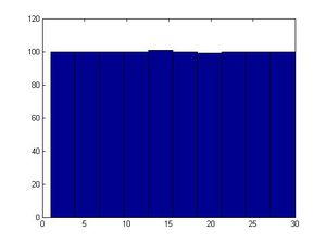
>>hist(x)

(Note: The semicolon after the x(ii)=mod(a*x(ii-1)+b,m) ensures that Matlab will not show the entire vector of x. It will instead calculate it internally and you will be able to work with it. Adding the semicolon to the end of this line reduces the run time significantly.)

This algorithm involves three integer parameters a, b, and m and an initial value, x₀ called seed. A sequence of numbers is defined by x(k+1) = a*x(k) + b mod m. Mod m means take the remainder after division by m.

Note: For some bad a and b, the histogram may not be uniformly distributed.

Example: a=13, b=0, m=31
The first 30 numbers in the sequence are a permutation of integers for 1 to 30 and then the sequence repeats itself. Values are between 0 and m-1. If the values are normalized by dividing by m-1, then the result is numbers uniformly distributed in the interval [0,1]. There are only a finite number of values (30 in this case). In Matlab, you can use function "hist(x)" to see if it is uniformly distributed.

Typically, it is good to choose m such that m is large, and m is prime. Careful selection of parameters helps generate relatively "random" output values, where it is harder to identify patterns.

For many years the “rand” function in Matlab used this algorithm with these parameters A=7^5=16807, b=0, m=2^31 -1=2147483647 – recommended in a 1988 paper by Park and Miller (Important part is that m should be large)

Inverse Transform Method

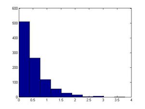
This method is useful for generating types of distribution other than uniform distribution, such as exponential distribution and normal distribution. Exponential distribution has the property that generated numbers are frequently close to 0. Normal distribution has the property that generated numbers are frequently close to its mean.

Theorem:
Take U ~ U[0,1] and let x=F^-1(U)
Then x has distribution function F(^.)
Where F(x) = P(X<=x) cdf; F^-1(U) denotes the inverse function of F(^.) Or that F(x)=U -> x=F^-1(U)

Proof of the theorem:
F(x)=P(X<=x)
=P(F^-1(U)<=x)
=P(F(F^-1(U))<=F(x)) #Applying F, which is monotonic, to both sides
=P(U<=F(x))
=F(x) #Because Pr(U<=y)= y,since U is uniform on the unit interval

F(^.) is a monotonic function, which is a function that strictly increasing or decreasing.

Example: [math]\displaystyle{ f(x) = \lambda e^{-\lambda x} }[/math]
[math]\displaystyle{ F(x)= \int_0^x f(x) dx }[/math]
[math]\displaystyle{ = \int_0^x \lambda e ^{-\lambda x}\ dx }[/math]
[math]\displaystyle{ = \frac{\lambda}{-\lambda}\, e^{-\lambda x}\, | \underset{0}{x} }[/math]
[math]\displaystyle{ = -e^{\lambda x} + e^0 }[/math]
[math]\displaystyle{ =1 - e^{- \lambda x} }[/math]

y=1-e^-λx;
1-y=e^-λx;
x=-ln(1-y)/λ;
y=-ln(1-x)/λ;
F^-1(x)=-ln(1-x)/λ;

Step 1: Draw U ~U[0,1];
Step 2: x=-ln(1-U)/ λ;

Example 2: Given a CDF of X: F(x) = x⁵, transform U~U[0,1]. Sol: Let y=x⁵, solve for x => x=y^(1/5) =>F^-1(x) = x^(1/5) Hence, to obtain a value of x from F(x), we first set u as an uniform distribution, then obtain the inverse function of F(x), and set x= u^(1/5)

In Matlab, you can use functions: "who" to see what variables you have defined "clear all" to clear all variables you have defined "close all" to close all figures

MatLab for Inverse Transform Method:

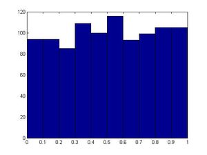
>>u=rand(1,1000)
>>hist(u)       #will generate a fairly uniform diagram

#let λ=2 in this example; however, you can make another value for λ
>>x=(-log(1-u))/2;
>>size(x)       #1000 in size 
>>figure
>>hist(x)       #exponential 

Limitations:
1. This method is flawed since not all functions are invertible nor monotonic.
2. It may be impractical since some CDF's and/or integrals are not easy to compute.

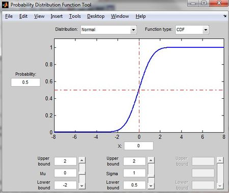
Probability Distribution Function Tool in MATLAB

>>disttool