ShakeDrop Regularization: Difference between revisions
| (73 intermediate revisions by 23 users not shown) | |||
| Line 1: | Line 1: | ||
=Introduction= | =Introduction= | ||
Current state of the art techniques for object classification are deep neural networks based on the residual block, first published by (He et al., 2016). This technique has been the foundation of several improved networks, including Wide ResNet (Zagoruyko & Komodakis, 2016), PyramdNet (Han et al., 2017) and ResNeXt (Xie et al., 2017). They have been further improved by regularization, such as Stochastic Depth (ResDrop) (Huang et al., 2016) and Shake-Shake (Gastaldi, 2017). Shake-Shake applied to | Current state of the art techniques for object classification are deep neural networks based on the residual block, first published by (He et al., 2016). This technique has been the foundation of several improved networks, including Wide ResNet (Zagoruyko & Komodakis, 2016), PyramdNet (Han et al., 2017) and ResNeXt (Xie et al., 2017). They have been further improved by regularization, such as Stochastic Depth (ResDrop) (Huang et al., 2016) and Shake-Shake (Gastaldi, 2017), which can avoid some problem like vanishing gradients. Shake-Shake applied to ResNeXt has achieved one of the lowest error rates on the CIFAR-10 and CIFAR-100 datasets. However, it is only applicable to multi-branch architectures and is not memory efficient since it requires two branches of residual blocks to apply. Note that the authors of Shake-Shake are rejecting the claim of their memory inefficiency. They claimed that there is no memory issue, just because there are <math>2\times</math> branches doesn't mean Shake-Shake needs <math>2\times</math> memory as it can use less memory to achieve the same performance. | ||
To address this problem, ShakeDrop regularization that can realize a similar disturbance to Shake-Shake on a single residual block is proposed.ShakeDrop disturbs learning more strongly by multiplying even a negative factor to the output of a convolutional layer in the forward training pass. In addition, a different factor from the forward pass is multiplied in the backward training pass. As a byproduct, however, learning process gets unstable. Moreover, they use ResDrop to stabilize the learning process. This paper seeks to formulate a general expansion of Shake-Shake that can be applied to any residual block based network. | |||
=Existing Methods= | =Existing Methods= | ||
| Line 6: | Line 8: | ||
'''Deep Approaches''' | '''Deep Approaches''' | ||
'''ResNet''', was the first use of residual blocks, a foundational feature in many modern state of the art convolution neural networks. They can be formulated as <math>G(x) = x + F(x)</math> where x and G(x) are the input and output of the residual block, and <math>F(x)</math> is the output of the residual block. A residual block typically performs a convolution operation and then passes the result plus its input onto the next block. | '''ResNet''', was the first use of residual blocks, a foundational feature in many modern state of the art convolution neural networks. They can be formulated as <math>G(x) = x + F(x)</math> where <math>x</math> and <math>G(x)</math> are the input and output of the residual block, and <math>F(x)</math> is the output of the residual branch on the residual block. A residual block typically performs a convolution operation and then passes the result plus its input onto the next block. | ||
The intuition behind Residual blocks: | |||
If the identity mapping is optimal, We can easily push the residuals to zero (F(x) = 0) than to fit an identity mapping (x, input=output) by a stack of non-linear layers. In simple language it is very easy to come up with a solution like F(x) =0 rather than F(x)=x using stack of non-linear cnn layers as function (Think about it). So, this function F(x) is what the authors called Residual function ([https://medium.com/@14prakash/understanding-and-implementing-architectures-of-resnet-and-resnext-for-state-of-the-art-image-cf51669e1624 Reference]). | |||
Residual blocks are used for two main reasons. First, as our networks become “deeper” and more flexible, we also need to take many more gradients during backpropagation. This exponentially increases the risk of vanishing gradients, particularly with state-of-the art structures. To counter this, residual layers pass entire layers – with the identity function applied – further down the network. Intuitively, this gives higher gradient values. Secondly, this gives the network another path to work on. If forced non-linearity is not an optimal choice, the network can bypass it through these residual blocks. In combination, residual blocks faciliate training of deep neural networks. | |||
[[File:ResidualBlock.png|580px|centre|thumb|An example of a simple residual block from Deep Residual Learning for Image Recognition by He et al., 2016]] | |||
ResNet is constructed out of a large number of these residual blocks sequentially stacked. It is interesting to note that having too many layers can cause overfitting, as pointed out by He et al. (2016) with the high error rates for the 1,202-layer ResNet on CIFAR datasets. Another paper (Veit et al., 2016) empirically showed that the cause of the high error rates can be mostly attributed to specific residual blocks whose channels increase greatly. | |||
ResNet is | '''PyramidNet''' is an important iteration that built on ResNet and WideResNet by gradually increasing channels on each residual block. The residual block is similar to those used in ResNet. It has been used to generate some of the first successful convolution neural networks with very large depth, at 272 layers. Amongst unmodified residual network architectures, it performs the best on the CIFAR datasets. | ||
[[File:ResidualBlockComparison.png|980px|centre|thumb|A simple illustration of different residual blocks from Deep Pyramidal Residual Networks by Han et al., 2017. The width of a block reflects the number of channels used in that layer.]] | |||
'''Non-Deep Approaches''' | '''Non-Deep Approaches''' | ||
'''Wide ResNet''' modified ResNet by increasing channels in each layer, having a wider and shallower structure. Similarly to PyramidNet, this architecture avoids some of the pitfalls in the | '''Wide ResNet''' modified ResNet by increasing channels in each layer, having a wider and shallower structure. Similarly to PyramidNet, this architecture avoids some of the pitfalls in the original formulation of ResNet. | ||
'''ResNeXt''' achieved performance beyond that of Wide ResNet with only a small increase in the number of parameters. It can be formulated as <math>G(x) = x + F_1(x)+F_2(x)</math>. In this case, <math>F_1(x)</math> and <math>F_2(x)</math> are the outputs of two paired convolution operations in a single residual block. The number of branches is not limited to 2, and will control the result of this network. | '''ResNeXt''' achieved performance beyond that of Wide ResNet with only a small increase in the number of parameters. It can be formulated as <math>G(x) = x + F_1(x)+F_2(x)</math>. In this case, <math>F_1(x)</math> and <math>F_2(x)</math> are the outputs of two paired convolution operations in a single residual block. The number of branches is not limited to 2, and will control the result of this network. | ||
'''Regularization Methods''' | [[File:SimplifiedResNeXt.png|600px|centre|thumb|Simplified ResNeXt Convolution Block. Yamada et al., 2018]] | ||
'''Regularization Methods For Residual Blocks''' | |||
'''Stochastic Depth''' works by randomly dropping paths in the residual blocks. On the <math>l^{th}</math> residual block the Stochastic Depth process is given as <math>G(x)=x+b_lF(x)</math> where <math>b_l \in \{0,1\}</math> is a Bernoulli random variable with probability <math>p_l</math>. Unlike sequential networks, there are many paths from the input to the output in these networks. By dropping some of the connections, the network is forced to flow through different paths to get the final deep layer representation. In a way it is similar to dropout, but for paths in multi-path networks. Using a constant value for <math>p_l</math> didn't work well, so instead a linear decay rule <math>p_l = 1 - \frac{l}{L}(1-p_L)</math> was used. In this equation, <math>L</math> is the number of layers, and <math>p_L</math> is the initial parameter. Essentially, the probability of a connection dropping in inversely proportional to the its depth in the network. | |||
''' | '''Shake-Shake''' is a regularization method that specifically improves the ResNeXt (multiple residual connections) architecture. It is given as <math>G(x)=x+\alpha F_1(x)+(1-\alpha)F_2(x)</math>, where <math>\alpha \in [0,1]</math> is a random coefficient. Essentially, one of the parallel residual connections is dropped in the forward direction. This is similar to stochastic depth regularization, but a residual path always exists. | ||
Moreover, on the backward pass a similar random variable <math>\beta</math> is used to independently drop paths for gradient flow. This has the effect of adding noise in the gradients update process and improved performance over the vanilla ResNeXt network. | |||
[[File:Paper 32.jpg|600px|centre|thumb| Shake-Shake (ResNeXt + Shake-Shake) (Gastaldi, 2017), in which some processing layers omitted for conciseness.]] | |||
=Proposed Method= | =Proposed Method= | ||
We give an intuitive interpretation of the forward pass of Shake-Shake regularization. To the best of our knowledge, it has not been given yet, while the phenomenon in the backward pass is experimentally investigated by Gastaldi (2017). In the forward pass, Shake-Shake interpolates the outputs of two residual branches with a random variable α that controls the degree of interpolation. As DeVries & Taylor (2017a) demonstrated that interpolation of two data in the feature space can synthesize reasonable augmented data, the interpolation of two residual blocks of Shake-Shake in the forward pass can be interpreted as synthesizing data. Use of a random variable α generates many different augmented data. On the other hand, in the backward pass, a different random variable β is used to disturb learning to make the network learnable long time. Gastaldi (2017) demonstrated how the difference between <math>\alpha</math> and <math>\beta</math> affects. | |||
The regularization mechanism of Shake-Shake relies on two or more residual branches, so that it can be applied only to 2-branch networks architectures. In addition, 2-branch network architectures consume more memory than 1-branch network architectures. One may think the number of learnable parameters of ResNeXt can be kept in 1-branch and 2-branch network architectures by controlling its cardinality and the number of channels (filters). For example, a 1-branch network (e.g., ResNeXt 1-64d) and its corresponding 2-branch network (e.g., ResNeXt 2-40d) have almost same number of learnable parameters. However, even so, it increases memory consumption due to the overhead to keep the inputs of residual blocks and so on. By comparing ResNeXt 1-64d and 2-40d, the latter requires more memory than the former by 8% in theory (for one layer) and by 11% in measured values (for 152 layers). | |||
This paper seeks to generalize the method proposed in Shake-Shake to be applied to any residual structure network. Shake-Shake. The initial formulation of 1-branch shake is <math>G(x) = x + \alpha F(x)</math>. In this case, <math>\alpha</math> is a coefficient that disturbs the forward pass, but is not necessarily constrained to be [0,1]. Another corresponding coefficient <math>\beta</math> is used in the backwards pass. Applying this simple adaptation of Shake-Shake on a 110-layer version of PyramidNet with <math>\alpha \in [0,1]</math> and <math>\beta \in [0,1]</math> performs abysmally, with an error rate of 77.99%. | This paper seeks to generalize the method proposed in Shake-Shake to be applied to any residual structure network. Shake-Shake. The initial formulation of 1-branch shake is <math>G(x) = x + \alpha F(x)</math>. In this case, <math>\alpha</math> is a coefficient that disturbs the forward pass, but is not necessarily constrained to be [0,1]. Another corresponding coefficient <math>\beta</math> is used in the backwards pass. Applying this simple adaptation of Shake-Shake on a 110-layer version of PyramidNet with <math>\alpha \in [0,1]</math> and <math>\beta \in [0,1]</math> performs abysmally, with an error rate of 77.99%. | ||
This failure is a result of the setup causing too much perturbation. A trick is needed to promote learning with large perturbations, to preserve the regularization effect. The idea of the authors is to borrow from ResDrop and combine that with Shake-Shake. This works by randomly deciding whether to apply 1-branch shake. This | This failure is a result of the setup causing too much perturbation. A trick is needed to promote learning with large perturbations, to preserve the regularization effect. The idea of the authors is to borrow from ResDrop and combine that with Shake-Shake. This works by randomly deciding whether to apply 1-branch shake. This creates in effect two networks, the original network without a regularization component, and a regularized network. When mixing up two networks, we expected the following effects: When the non regularized network is selected, learning is promoted; when the perturbed network is selected, learning is disturbed. Achieving good performance requires a balance between the two. | ||
'''ShakeDrop''' is given as | '''ShakeDrop''' is given as | ||
<div align="center"> | |||
<math>G(x) = x + (b_l + \alpha - b_l \alpha)F(x)</math>, | <math>G(x) = x + (b_l + \alpha - b_l \alpha)F(x)</math>, | ||
</div> | |||
where <math>b_l</math> is a Bernoulli random variable following the linear decay rule used in Stochastic Depth. An alternative presentation is | where <math>b_l</math> is a Bernoulli random variable following the linear decay rule used in Stochastic Depth. An alternative presentation is | ||
<math>G(x) = x + F(x) | <div align="center"> | ||
<math> | |||
G(x) = \begin{cases} | |||
x + F(x) ~~ \text{if } b_l = 1 \\ | |||
x + \alpha F(x) ~~ \text{otherwise} | |||
\end{cases} | |||
</math> | |||
</div> | |||
<math> | If <math>b_l = 1</math> then ShakeDrop is equivalent to the original network, otherwise it is the network + 1-branch Shake. The authors also found that the linear decay rule of ResDrop works well, compared with the uniform rule. Regardless of the value of <math>\beta</math> on the backwards pass, network weights will be updated. | ||
=Experiments= | |||
'''Parameter Search''' | |||
The authors experiments began with a hyperparameter search utilizing ShakeDrop on pyramidal networks. The PyramidNet used was made up of a total of 110 layers which included a convolutional layer and a final fully connected layer. It had 54 additive pyramidal residual blocks and the final residual block had 286 channels. The results of this search are presented below. | |||
[[File:ShakeDropHyperParameterSearch.png|600px|centre|thumb|Average Top-1 errors (%) of “PyramidNet + ShakeDrop” with several ranges of parameters of 4 runs at the final (300th) epoch on CIFAR-100 dataset in the “Batch” level. In some settings, it is equivalent to PyramidNet and PyramidDrop. Borrowed from ShakeDrop Regularization by Yamada et al., 2018.]] | |||
The setting that are used throughout the rest of the experiments are then <math>\alpha \in [-1,1]</math> and <math>\beta \in [0,1]</math>. Cases H and F outperform PyramidNet, suggesting that the strong perturbations imposed by ShakeDrop are functioning as intended. However, fully applying the perturbations in the backwards pass appears to destabilize the network, resulting in performance that is worse than standard PyramidNet. | |||
[[File:ParameterUpdateShakeDrop.png|400px|centre]] | |||
Following this initial parameter decision, the authors tested 4 different strategies for parameter update among "Batch" (same coefficients for all images in minibatch for each residual block), "Image" (same scaling coefficients for each image for each residual block), "Channel" (same scaling coefficients for each element for each residual block), and "Pixel" (same scaling coefficients for each element for each residual block). While Pixel was the best in terms of error rate, it is not very memory efficient, so Image was selected as it had the second best performance without the memory drawback. | |||
'''Comparison with Regularization Methods''' | |||
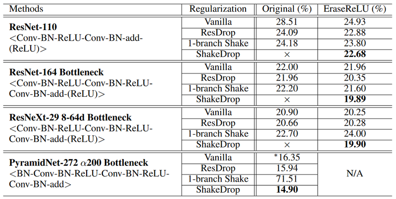
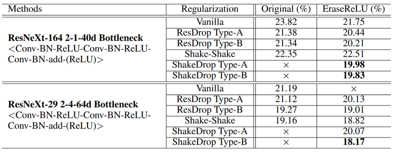
For these experiments, there are a few modifications that were made to assist with training. For ResNeXt, the EraseRelu formulation has each residual block ends in batch normalization. The Wide ResNet also is compared between vanilla with batch normalization and without. Batch normalization keeps the outputs of residual blocks in a certain range, as otherwise <math>\alpha</math> and <math>\beta</math> could cause perturbations that are too large, causing divergent learning. There is also a comparison of ResDrop/ShakeDrop Type A (where the regularization unit is inserted before the add unit for a residual branch) and after (where the regularization unit is inserted after the add unit for a residual branch). | |||
These experiments are performed on the CIFAR-100 dataset. | |||
[[File:ShakeDropArchitectureComparison1.png|800px|centre|thumb|]] | |||
[[File:ShakeDropArchitectureComparison2.png|800px|centre|thumb|]] | |||
[[File:ShakeDropArchitectureComparison3.png|800px|centre|thumb|]] | |||
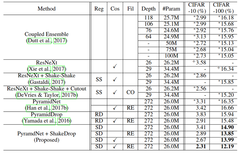
For a final round of testing, the training setup was modified to incorporate other techniques used in state of the art methods. For most of the tests, the learning rate for the 300 epoch version started at 0.1 and decayed by a factor of 0.1 1/2 & 3/4 of the way through training. The alternative was cosine annealing, based on the presentation by Loshchilov and Hutter in their paper SGDR: Stochastic Gradient Descent with Warm Restarts. This is indicated in the Cos column, with a check indicating cosine annealing. | |||
[[File:CosineAnnealing.png|400px|centre|thumb|]] | |||
The Reg column indicates the regularization method used, either none, ResDrop (RD), Shake-Shake (SS), or ShakeDrop (SD). Fianlly, the Fil Column determines the type of data augmentation used, either none, cutout (CO) (DeVries & Taylor, 2017b), or Random Erasing (RE) (Zhong et al., 2017). | |||
[[File:ShakeDropComparison.png|800px|centre|thumb|Top-1 Errors (%) at final epoch on CIFAR-10/100 datasets]] | |||
'''State-of-the-Art Comparisons''' | |||
A direct comparison with state of the art methods is favorable for this new method. | |||
# Fair comparison of ResNeXt + Shake-Shake with PyramidNet + ShakeDrop gives an improvement of 0.19% on CIFAR-10 and 1.86% on CIFAR-100. Under these conditions, the final error rate is then 2.67% for CIFAR-10 and 13.99% for CIFAR-100. | |||
# Fair comparison of ResNeXt + Shake-Shake + Cutout with PyramidNet + ShakeDrop + Random Erasing gives an improvement of 0.25% on CIFAR-10 and 3.01% on CIFAR 100. Under these conditions, the final error rate is then 2.31% for CIFAR-10 and 12.19% for CIFAR-100. | |||
# Comparison with the state-of-the-arts, PyramidNet + ShakeDrop gives an improvement of 0.25% on CIFAR-10 than ResNeXt + Shake-Shake + Cutout, PyramidNet + ShakeDrop gives an improvement of 2.85% on CIFAR-100 than Coupled Ensemble. | |||
=Implementation details= | |||
'''CIFAR-10/100 datasets''' | |||
All the images in these datasets were color normalized and then horizontally flipped with a probability of 50%. All of then then were zero padded to have a dimentionality of 40 by 40 pixels. | |||
'''ImageNet dataset''' | |||
The data augmentation process included a random distortion conditioned to an aspect ratio, random crop down to a 224x224 pixels, random horizontal flipping with 50% of probability. | |||
=Conclusion= | |||
The paper proposes a new form of regularization that is an extension of "Shake-Shake" regularization [Gastaldi, 2017]. The original "shake-shake" proposes using two residual paths adding to the same output, and during training, considering different randomly selected convex combinations of the two paths (while using an equally weighted combination at test time). This paper contends that this requires additional memory, and attempts to achieve similar regularization with a single path. To do so, they train a network with a single residual path, where the residual is included without attenuation in some cases with some fixed probability, and attenuated randomly (or even inverted) in others. The paper contends that this achieves superior performance than choosing simply a random attenuation for every sample (although, this can be seen as choosing an attenuation under a distribution with some fixed probability mass. | |||
Their stochastic regularization method, ShakeDrop, which outperforms previous state of the art methods while maintaining similar memory efficiency. It demonstrates that heavily perturbing a network can help to overcome issues with overfitting. It is also an effective way to regularize residual networks for image classification. The method was tested by CIFAR-10/100 and Tiny ImageNet datasets and showed great performance. | |||
=Critique= | |||
The novelty of this paper is low as pointed out by the reviewers. Also, there is a confusion whether or not the results could be replicated as <math>\alpha</math> and <math>\beta</math> are choosen randomly. The proposed ShakeDrop regularization is essentially a combination of the PyramidDrop and Shake-Shake regularization. The most surprising part is that the forward weight can be negative thus inverting the output of a convolution. The mathematical justification for ShakeDrop regularization is limited, relying on intuition and empirical evidence instead. | |||
One downside of this methods (as was identified in the presentation as well) is that the training for cosine annealing variation of the model takes 1800 epochs which is time intensive compared to other methods that were compared as baselines. This can limit practical implementation of this algorithm. | |||
As pointed out from the above, the method basically relies heavily on the intuition. This means that the performance of the algorithm can not been extended beyond the CIFAR dataset and can vary a lot depending on the characteristics of data sets that users are performing, with some exaggeration. However, the performance is still impressive since it performs better than known algorithms. It is not clear as to how the proposed technique would work with a non-residual architecture. | |||
It lacks conclusive proof that "shake-drop" is a generically useful regularization technique. For one, the method is evaluated only on small toy-datasets: CIFAR-10 and CIFAR-100. Evaluation on Imagenet perhaps would have been valuable. There is also another dataset that would of been good to try SVHN. Overall I believe the impact of this beyond CIFAR is unclear. | |||
=References= | =References= | ||
[Yamada et al., 2018] Yamada Y, Iwamura M, Kise K. ShakeDrop regularization. arXiv preprint arXiv:1802.02375. 2018 Feb 7. | |||
[He et al., 2016] Kaiming He, Xiangyu Zhang, Shaoqing Ren, and Jian Sun. Deep residual learning for image recognition. In Proc. CVPR, 2016. | [He et al., 2016] Kaiming He, Xiangyu Zhang, Shaoqing Ren, and Jian Sun. Deep residual learning for image recognition. In Proc. CVPR, 2016. | ||
| Line 58: | Line 152: | ||
[Gastaldi, 2017] Xavier Gastaldi. Shake-shake regularization. arXiv preprint arXiv:1705.07485v2, 2017. | [Gastaldi, 2017] Xavier Gastaldi. Shake-shake regularization. arXiv preprint arXiv:1705.07485v2, 2017. | ||
[Loshilov & Hutter, 2016] Ilya Loshchilov and Frank Hutter. Sgdr: Stochastic gradient descent with warm restarts. arXiv preprint arXiv:1608.03983, 2016. | |||
[DeVries & Taylor, 2017b] Terrance DeVries and Graham W. Taylor. Improved regularization of convolutional neural networks with cutout. arXiv preprint arXiv:1708.04552, 2017b. | |||
[Zhong et al., 2017] Zhun Zhong, Liang Zheng, Guoliang Kang, Shaozi Li, and Yi Yang. Random erasing data augmentation. arXiv preprint arXiv:1708.04896, 2017. | |||
[Dutt et al., 2017] Anuvabh Dutt, Denis Pellerin, and Georges Qunot. Coupled ensembles of neural networks. arXiv preprint 1709.06053v1, 2017. | |||
[Veit et al., 2016] Andreas Veit, Michael J Wilber, and Serge Belongie. Residual networks behave like ensembles of relatively shallow networks. Advances in Neural Information Processing Systems 29, 2016. | |||
Latest revision as of 00:34, 17 December 2018
Introduction
Current state of the art techniques for object classification are deep neural networks based on the residual block, first published by (He et al., 2016). This technique has been the foundation of several improved networks, including Wide ResNet (Zagoruyko & Komodakis, 2016), PyramdNet (Han et al., 2017) and ResNeXt (Xie et al., 2017). They have been further improved by regularization, such as Stochastic Depth (ResDrop) (Huang et al., 2016) and Shake-Shake (Gastaldi, 2017), which can avoid some problem like vanishing gradients. Shake-Shake applied to ResNeXt has achieved one of the lowest error rates on the CIFAR-10 and CIFAR-100 datasets. However, it is only applicable to multi-branch architectures and is not memory efficient since it requires two branches of residual blocks to apply. Note that the authors of Shake-Shake are rejecting the claim of their memory inefficiency. They claimed that there is no memory issue, just because there are [math]\displaystyle{ 2\times }[/math] branches doesn't mean Shake-Shake needs [math]\displaystyle{ 2\times }[/math] memory as it can use less memory to achieve the same performance.
To address this problem, ShakeDrop regularization that can realize a similar disturbance to Shake-Shake on a single residual block is proposed.ShakeDrop disturbs learning more strongly by multiplying even a negative factor to the output of a convolutional layer in the forward training pass. In addition, a different factor from the forward pass is multiplied in the backward training pass. As a byproduct, however, learning process gets unstable. Moreover, they use ResDrop to stabilize the learning process. This paper seeks to formulate a general expansion of Shake-Shake that can be applied to any residual block based network.
Existing Methods
Deep Approaches
ResNet, was the first use of residual blocks, a foundational feature in many modern state of the art convolution neural networks. They can be formulated as [math]\displaystyle{ G(x) = x + F(x) }[/math] where [math]\displaystyle{ x }[/math] and [math]\displaystyle{ G(x) }[/math] are the input and output of the residual block, and [math]\displaystyle{ F(x) }[/math] is the output of the residual branch on the residual block. A residual block typically performs a convolution operation and then passes the result plus its input onto the next block.
The intuition behind Residual blocks: If the identity mapping is optimal, We can easily push the residuals to zero (F(x) = 0) than to fit an identity mapping (x, input=output) by a stack of non-linear layers. In simple language it is very easy to come up with a solution like F(x) =0 rather than F(x)=x using stack of non-linear cnn layers as function (Think about it). So, this function F(x) is what the authors called Residual function (Reference).
Residual blocks are used for two main reasons. First, as our networks become “deeper” and more flexible, we also need to take many more gradients during backpropagation. This exponentially increases the risk of vanishing gradients, particularly with state-of-the art structures. To counter this, residual layers pass entire layers – with the identity function applied – further down the network. Intuitively, this gives higher gradient values. Secondly, this gives the network another path to work on. If forced non-linearity is not an optimal choice, the network can bypass it through these residual blocks. In combination, residual blocks faciliate training of deep neural networks.
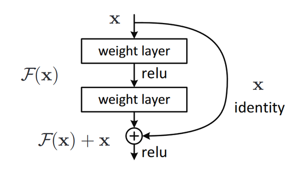
ResNet is constructed out of a large number of these residual blocks sequentially stacked. It is interesting to note that having too many layers can cause overfitting, as pointed out by He et al. (2016) with the high error rates for the 1,202-layer ResNet on CIFAR datasets. Another paper (Veit et al., 2016) empirically showed that the cause of the high error rates can be mostly attributed to specific residual blocks whose channels increase greatly.
PyramidNet is an important iteration that built on ResNet and WideResNet by gradually increasing channels on each residual block. The residual block is similar to those used in ResNet. It has been used to generate some of the first successful convolution neural networks with very large depth, at 272 layers. Amongst unmodified residual network architectures, it performs the best on the CIFAR datasets.

Non-Deep Approaches
Wide ResNet modified ResNet by increasing channels in each layer, having a wider and shallower structure. Similarly to PyramidNet, this architecture avoids some of the pitfalls in the original formulation of ResNet.
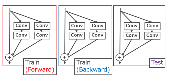
ResNeXt achieved performance beyond that of Wide ResNet with only a small increase in the number of parameters. It can be formulated as [math]\displaystyle{ G(x) = x + F_1(x)+F_2(x) }[/math]. In this case, [math]\displaystyle{ F_1(x) }[/math] and [math]\displaystyle{ F_2(x) }[/math] are the outputs of two paired convolution operations in a single residual block. The number of branches is not limited to 2, and will control the result of this network.
Regularization Methods For Residual Blocks
Stochastic Depth works by randomly dropping paths in the residual blocks. On the [math]\displaystyle{ l^{th} }[/math] residual block the Stochastic Depth process is given as [math]\displaystyle{ G(x)=x+b_lF(x) }[/math] where [math]\displaystyle{ b_l \in \{0,1\} }[/math] is a Bernoulli random variable with probability [math]\displaystyle{ p_l }[/math]. Unlike sequential networks, there are many paths from the input to the output in these networks. By dropping some of the connections, the network is forced to flow through different paths to get the final deep layer representation. In a way it is similar to dropout, but for paths in multi-path networks. Using a constant value for [math]\displaystyle{ p_l }[/math] didn't work well, so instead a linear decay rule [math]\displaystyle{ p_l = 1 - \frac{l}{L}(1-p_L) }[/math] was used. In this equation, [math]\displaystyle{ L }[/math] is the number of layers, and [math]\displaystyle{ p_L }[/math] is the initial parameter. Essentially, the probability of a connection dropping in inversely proportional to the its depth in the network.
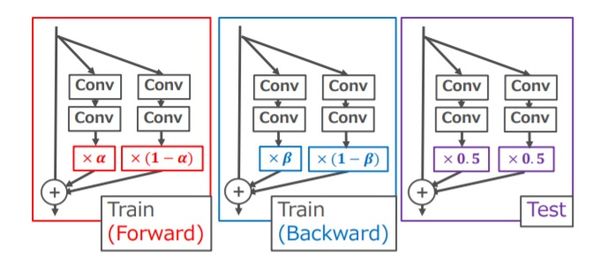
Shake-Shake is a regularization method that specifically improves the ResNeXt (multiple residual connections) architecture. It is given as [math]\displaystyle{ G(x)=x+\alpha F_1(x)+(1-\alpha)F_2(x) }[/math], where [math]\displaystyle{ \alpha \in [0,1] }[/math] is a random coefficient. Essentially, one of the parallel residual connections is dropped in the forward direction. This is similar to stochastic depth regularization, but a residual path always exists. Moreover, on the backward pass a similar random variable [math]\displaystyle{ \beta }[/math] is used to independently drop paths for gradient flow. This has the effect of adding noise in the gradients update process and improved performance over the vanilla ResNeXt network.
Proposed Method
We give an intuitive interpretation of the forward pass of Shake-Shake regularization. To the best of our knowledge, it has not been given yet, while the phenomenon in the backward pass is experimentally investigated by Gastaldi (2017). In the forward pass, Shake-Shake interpolates the outputs of two residual branches with a random variable α that controls the degree of interpolation. As DeVries & Taylor (2017a) demonstrated that interpolation of two data in the feature space can synthesize reasonable augmented data, the interpolation of two residual blocks of Shake-Shake in the forward pass can be interpreted as synthesizing data. Use of a random variable α generates many different augmented data. On the other hand, in the backward pass, a different random variable β is used to disturb learning to make the network learnable long time. Gastaldi (2017) demonstrated how the difference between [math]\displaystyle{ \alpha }[/math] and [math]\displaystyle{ \beta }[/math] affects.
The regularization mechanism of Shake-Shake relies on two or more residual branches, so that it can be applied only to 2-branch networks architectures. In addition, 2-branch network architectures consume more memory than 1-branch network architectures. One may think the number of learnable parameters of ResNeXt can be kept in 1-branch and 2-branch network architectures by controlling its cardinality and the number of channels (filters). For example, a 1-branch network (e.g., ResNeXt 1-64d) and its corresponding 2-branch network (e.g., ResNeXt 2-40d) have almost same number of learnable parameters. However, even so, it increases memory consumption due to the overhead to keep the inputs of residual blocks and so on. By comparing ResNeXt 1-64d and 2-40d, the latter requires more memory than the former by 8% in theory (for one layer) and by 11% in measured values (for 152 layers).
This paper seeks to generalize the method proposed in Shake-Shake to be applied to any residual structure network. Shake-Shake. The initial formulation of 1-branch shake is [math]\displaystyle{ G(x) = x + \alpha F(x) }[/math]. In this case, [math]\displaystyle{ \alpha }[/math] is a coefficient that disturbs the forward pass, but is not necessarily constrained to be [0,1]. Another corresponding coefficient [math]\displaystyle{ \beta }[/math] is used in the backwards pass. Applying this simple adaptation of Shake-Shake on a 110-layer version of PyramidNet with [math]\displaystyle{ \alpha \in [0,1] }[/math] and [math]\displaystyle{ \beta \in [0,1] }[/math] performs abysmally, with an error rate of 77.99%.
This failure is a result of the setup causing too much perturbation. A trick is needed to promote learning with large perturbations, to preserve the regularization effect. The idea of the authors is to borrow from ResDrop and combine that with Shake-Shake. This works by randomly deciding whether to apply 1-branch shake. This creates in effect two networks, the original network without a regularization component, and a regularized network. When mixing up two networks, we expected the following effects: When the non regularized network is selected, learning is promoted; when the perturbed network is selected, learning is disturbed. Achieving good performance requires a balance between the two.
ShakeDrop is given as
[math]\displaystyle{ G(x) = x + (b_l + \alpha - b_l \alpha)F(x) }[/math],
where [math]\displaystyle{ b_l }[/math] is a Bernoulli random variable following the linear decay rule used in Stochastic Depth. An alternative presentation is
[math]\displaystyle{ G(x) = \begin{cases} x + F(x) ~~ \text{if } b_l = 1 \\ x + \alpha F(x) ~~ \text{otherwise} \end{cases} }[/math]
If [math]\displaystyle{ b_l = 1 }[/math] then ShakeDrop is equivalent to the original network, otherwise it is the network + 1-branch Shake. The authors also found that the linear decay rule of ResDrop works well, compared with the uniform rule. Regardless of the value of [math]\displaystyle{ \beta }[/math] on the backwards pass, network weights will be updated.
Experiments
Parameter Search
The authors experiments began with a hyperparameter search utilizing ShakeDrop on pyramidal networks. The PyramidNet used was made up of a total of 110 layers which included a convolutional layer and a final fully connected layer. It had 54 additive pyramidal residual blocks and the final residual block had 286 channels. The results of this search are presented below.
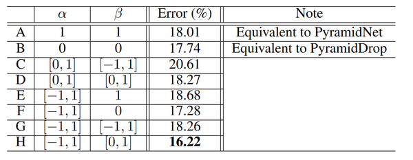
The setting that are used throughout the rest of the experiments are then [math]\displaystyle{ \alpha \in [-1,1] }[/math] and [math]\displaystyle{ \beta \in [0,1] }[/math]. Cases H and F outperform PyramidNet, suggesting that the strong perturbations imposed by ShakeDrop are functioning as intended. However, fully applying the perturbations in the backwards pass appears to destabilize the network, resulting in performance that is worse than standard PyramidNet.
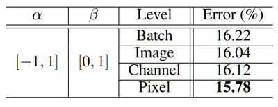
Following this initial parameter decision, the authors tested 4 different strategies for parameter update among "Batch" (same coefficients for all images in minibatch for each residual block), "Image" (same scaling coefficients for each image for each residual block), "Channel" (same scaling coefficients for each element for each residual block), and "Pixel" (same scaling coefficients for each element for each residual block). While Pixel was the best in terms of error rate, it is not very memory efficient, so Image was selected as it had the second best performance without the memory drawback.
Comparison with Regularization Methods
For these experiments, there are a few modifications that were made to assist with training. For ResNeXt, the EraseRelu formulation has each residual block ends in batch normalization. The Wide ResNet also is compared between vanilla with batch normalization and without. Batch normalization keeps the outputs of residual blocks in a certain range, as otherwise [math]\displaystyle{ \alpha }[/math] and [math]\displaystyle{ \beta }[/math] could cause perturbations that are too large, causing divergent learning. There is also a comparison of ResDrop/ShakeDrop Type A (where the regularization unit is inserted before the add unit for a residual branch) and after (where the regularization unit is inserted after the add unit for a residual branch).
These experiments are performed on the CIFAR-100 dataset.

For a final round of testing, the training setup was modified to incorporate other techniques used in state of the art methods. For most of the tests, the learning rate for the 300 epoch version started at 0.1 and decayed by a factor of 0.1 1/2 & 3/4 of the way through training. The alternative was cosine annealing, based on the presentation by Loshchilov and Hutter in their paper SGDR: Stochastic Gradient Descent with Warm Restarts. This is indicated in the Cos column, with a check indicating cosine annealing.

The Reg column indicates the regularization method used, either none, ResDrop (RD), Shake-Shake (SS), or ShakeDrop (SD). Fianlly, the Fil Column determines the type of data augmentation used, either none, cutout (CO) (DeVries & Taylor, 2017b), or Random Erasing (RE) (Zhong et al., 2017).
State-of-the-Art Comparisons
A direct comparison with state of the art methods is favorable for this new method.
- Fair comparison of ResNeXt + Shake-Shake with PyramidNet + ShakeDrop gives an improvement of 0.19% on CIFAR-10 and 1.86% on CIFAR-100. Under these conditions, the final error rate is then 2.67% for CIFAR-10 and 13.99% for CIFAR-100.
- Fair comparison of ResNeXt + Shake-Shake + Cutout with PyramidNet + ShakeDrop + Random Erasing gives an improvement of 0.25% on CIFAR-10 and 3.01% on CIFAR 100. Under these conditions, the final error rate is then 2.31% for CIFAR-10 and 12.19% for CIFAR-100.
- Comparison with the state-of-the-arts, PyramidNet + ShakeDrop gives an improvement of 0.25% on CIFAR-10 than ResNeXt + Shake-Shake + Cutout, PyramidNet + ShakeDrop gives an improvement of 2.85% on CIFAR-100 than Coupled Ensemble.
Implementation details
CIFAR-10/100 datasets
All the images in these datasets were color normalized and then horizontally flipped with a probability of 50%. All of then then were zero padded to have a dimentionality of 40 by 40 pixels.
ImageNet dataset
The data augmentation process included a random distortion conditioned to an aspect ratio, random crop down to a 224x224 pixels, random horizontal flipping with 50% of probability.
Conclusion
The paper proposes a new form of regularization that is an extension of "Shake-Shake" regularization [Gastaldi, 2017]. The original "shake-shake" proposes using two residual paths adding to the same output, and during training, considering different randomly selected convex combinations of the two paths (while using an equally weighted combination at test time). This paper contends that this requires additional memory, and attempts to achieve similar regularization with a single path. To do so, they train a network with a single residual path, where the residual is included without attenuation in some cases with some fixed probability, and attenuated randomly (or even inverted) in others. The paper contends that this achieves superior performance than choosing simply a random attenuation for every sample (although, this can be seen as choosing an attenuation under a distribution with some fixed probability mass.
Their stochastic regularization method, ShakeDrop, which outperforms previous state of the art methods while maintaining similar memory efficiency. It demonstrates that heavily perturbing a network can help to overcome issues with overfitting. It is also an effective way to regularize residual networks for image classification. The method was tested by CIFAR-10/100 and Tiny ImageNet datasets and showed great performance.
Critique
The novelty of this paper is low as pointed out by the reviewers. Also, there is a confusion whether or not the results could be replicated as [math]\displaystyle{ \alpha }[/math] and [math]\displaystyle{ \beta }[/math] are choosen randomly. The proposed ShakeDrop regularization is essentially a combination of the PyramidDrop and Shake-Shake regularization. The most surprising part is that the forward weight can be negative thus inverting the output of a convolution. The mathematical justification for ShakeDrop regularization is limited, relying on intuition and empirical evidence instead.
One downside of this methods (as was identified in the presentation as well) is that the training for cosine annealing variation of the model takes 1800 epochs which is time intensive compared to other methods that were compared as baselines. This can limit practical implementation of this algorithm.
As pointed out from the above, the method basically relies heavily on the intuition. This means that the performance of the algorithm can not been extended beyond the CIFAR dataset and can vary a lot depending on the characteristics of data sets that users are performing, with some exaggeration. However, the performance is still impressive since it performs better than known algorithms. It is not clear as to how the proposed technique would work with a non-residual architecture. It lacks conclusive proof that "shake-drop" is a generically useful regularization technique. For one, the method is evaluated only on small toy-datasets: CIFAR-10 and CIFAR-100. Evaluation on Imagenet perhaps would have been valuable. There is also another dataset that would of been good to try SVHN. Overall I believe the impact of this beyond CIFAR is unclear.
References
[Yamada et al., 2018] Yamada Y, Iwamura M, Kise K. ShakeDrop regularization. arXiv preprint arXiv:1802.02375. 2018 Feb 7.
[He et al., 2016] Kaiming He, Xiangyu Zhang, Shaoqing Ren, and Jian Sun. Deep residual learning for image recognition. In Proc. CVPR, 2016.
[Zagoruyko & Komodakis, 2016] Sergey Zagoruyko and Nikos Komodakis. Wide residual networks. In Proc. BMVC, 2016.
[Han et al., 2017] Dongyoon Han, Jiwhan Kim, and Junmo Kim. Deep pyramidal residual networks. In Proc. CVPR, 2017a.
[Xie et al., 2017] Saining Xie, Ross Girshick, Piotr Dollar, Zhuowen Tu, and Kaiming He. Aggregated residual transformations for deep neural networks. In Proc. CVPR, 2017.
[Huang et al., 2016] Gao Huang, Yu Sun, Zhuang Liu, Daniel Sedra, and Kilian Weinberger. Deep networks with stochastic depth. arXiv preprint arXiv:1603.09382v3, 2016.
[Gastaldi, 2017] Xavier Gastaldi. Shake-shake regularization. arXiv preprint arXiv:1705.07485v2, 2017.
[Loshilov & Hutter, 2016] Ilya Loshchilov and Frank Hutter. Sgdr: Stochastic gradient descent with warm restarts. arXiv preprint arXiv:1608.03983, 2016.
[DeVries & Taylor, 2017b] Terrance DeVries and Graham W. Taylor. Improved regularization of convolutional neural networks with cutout. arXiv preprint arXiv:1708.04552, 2017b.
[Zhong et al., 2017] Zhun Zhong, Liang Zheng, Guoliang Kang, Shaozi Li, and Yi Yang. Random erasing data augmentation. arXiv preprint arXiv:1708.04896, 2017.
[Dutt et al., 2017] Anuvabh Dutt, Denis Pellerin, and Georges Qunot. Coupled ensembles of neural networks. arXiv preprint 1709.06053v1, 2017.
[Veit et al., 2016] Andreas Veit, Michael J Wilber, and Serge Belongie. Residual networks behave like ensembles of relatively shallow networks. Advances in Neural Information Processing Systems 29, 2016.