stat946w18/Wavelet Pooling For Convolutional Neural Networks: Difference between revisions
(Technical) |
|||
| (43 intermediate revisions by 19 users not shown) | |||
| Line 1: | Line 1: | ||
== Introduction, Important Terms and Brief Summary== | == Introduction, Important Terms and Brief Summary== | ||
This paper focuses on the following important techniques: | This paper focuses on the following important techniques: | ||
1) Convolutional Neural Nets (CNN): These are networks with layered structures that conform to the shape of inputs and consistently obtain high accuracies in the classification of images and objects. Researchers continue to focus on CNN to improve their performances. | 1) Convolutional Neural Nets (CNN): These are networks with layered structures that conform to the shape of inputs rather than vector-based features and consistently obtain high accuracies in the classification of images and objects. Researchers continue to focus on CNN to improve their performances. | ||
2) Pooling: Pooling subsamples the results of the convolution layers and gradually reduces spatial dimensions of the data throughout the network. It is done to reduce parameters, increase computational efficiency and regulate overfitting. | 2) Pooling: Pooling subsamples the results of the convolution layers and gradually reduces spatial dimensions of the data throughout the network. It is done to reduce parameters, increase computational efficiency and regulate overfitting. | ||
Some of pooling methods, including max pooling and average pooling, are deterministic. | Some of the pooling methods, including max pooling and average pooling, are deterministic. Deterministic pooling methods are efficient and simple, but can hinder the potential for optimal network learning. In contrast, mixed pooling and stochastic pooling use a probabilistic approach, which can address some problems of deterministic methods. The neighborhood approach is used in all the mentioned pooling methods due to its simplicity and efficiency. Nevertheless, the approach can cause edge halos, blurring, and aliasing which need to be minimized. This paper introduces wavelet pooling, which uses a second-level wavelet decomposition to subsample features. The nearest neighbor interpolation is replaced by an organic, subband method that more accurately represents the feature contents with fewer artifacts. The method decomposes features into a second level decomposition and discards first level subbands to reduce feature dimensions. This method is compared to other state-of-the-art pooling methods to demonstrate superior results. Tests are conducted on benchmark classification tests like MNIST, CIFAR10, SHVN and KDEF. | ||
For further information on wavelets, follow this link to MathWorks' [https://www.mathworks.com/videos/understanding-wavelets-part-1-what-are-wavelets-121279.html Understanding Wavelets] video series. | |||
== Intuition == | == Intuition == | ||
Convolutional networks commonly employ convolutional layers to extract features and use pooling methods for spatial dimensionality reduction. In this study, wavelet pooling is introduced as an alternative to traditional neighborhood pooling by providing a more structural feature dimension reduction method. Max pooling is addressed to have over-fitting problems and average pooling is mentioned to smooth | Convolutional networks commonly employ convolutional layers to extract features and use pooling methods for spatial dimensionality reduction. In this study, wavelet pooling is introduced as an alternative to traditional neighborhood pooling by providing a more structural feature dimension reduction method. Max pooling is addressed to have over-fitting problems and average pooling is mentioned to smooth out or 'dilute' details in features. | ||
Pooling is often introduced within networks to ensure local invariance to prevent overfitting due to small transitional shifts within an image. Despite the effectiveness of traditional pooling methods such as max pooling introduce this translational invariance by discarding information using methods analogous to nearest neighbour interpolation. With the hope of providing a more organic way of pooling, the authors leverage all information within cells inputted within a pooling operation with the hope that the resulting dim-reduced features are able to contain information from all high level cells using various dot products. | |||
== History == | == History == | ||
A history of different pooling methods have been introduced and referenced in this study: | A history of different pooling methods have been introduced and referenced in this study: | ||
* | * Manual subsampling at 1979 | ||
* Max pooling at 1992 | * Max pooling at 1992 | ||
* Mixed pooling at 2014 | * Mixed pooling at 2014 | ||
* | * Pooling methods with probabilistic approaches at 2014 and 2015 | ||
== Background == | == Background == | ||
Average Pooling and Max Pooling are well known pooling methods and are popular techniques used in the literature. While these methods are simple and effective, | Average Pooling and Max Pooling are well-known pooling methods and are popular techniques used in the literature. These pooling methods reduce input data dimensionality by taking the maximum value or the average value of specific areas and condense them into one single value. While these methods are simple and effective, they still have some limitations. The authors identify the following limitations: | ||
'''Limitations of Max Pooling and Average Pooling''' | '''Limitations of Max Pooling and Average Pooling''' | ||
'''Max pooling''': takes the maximum value of a region | '''Max pooling''': takes the maximum value of a region <math>R_{ij} </math> and selects it to obtain a condensed feature map. It can '''erase the details''' of the image (happens if the main details have less intensity than the insignificant details) and also commonly '''over-fits''' the training data. The max-pooling is defined as: | ||
\begin{align} | \begin{align} | ||
| Line 37: | Line 36: | ||
\end{align} | \end{align} | ||
'''Average pooling''': calculates the average value of a region and selects it to obtain a condensed feature map. Depending on the data, this method can '''dilute pertinent details''' from an image (happens for data with values much lower than significant details) The avg-pooling is defined as: | '''Average pooling''': calculates the average value of a region and selects it to obtain a condensed feature map. Depending on the data, this method can '''dilute pertinent details''' from an image (happens for data with values much lower than the significant details) The avg-pooling is defined as: | ||
\begin{align} | \begin{align} | ||
| Line 43: | Line 42: | ||
\end{align} | \end{align} | ||
Where <math>a_{kij}</math> is the output activation of the <math>k^{th}</math> feature map at <math>(i,j)</math>, <math>a_{ | Where <math>a_{kij}</math> is the output activation of the <math>k^{th}</math> feature map at <math>(i,j)</math>, <math>a_{kpq}</math> is the input activation at | ||
<math>(p,q)</math> within <math>R_{ij}</math>, and <math>|R_{ij}|</math> is the size of the pooling region. | <math>(p,q)</math> within <math>R_{ij}</math>, and <math>|R_{ij}|</math> is the size of the pooling region. Figure 1 gives a quick visual example of max and average pooling: | ||
[[File: pooling.png| 700px|center]] | |||
Figure 2 provides an example of the weaknesses of these two methods using toy images: | |||
[[File: fig0001.PNG| 700px|center]] | [[File: fig0001.PNG| 700px|center]] | ||
| Line 51: | Line 54: | ||
'''How the researchers try to '''combat these issues'''?''' | '''How the researchers try to '''combat these issues'''?''' | ||
Using '''probabilistic pooling methods''' such as: | Using '''probabilistic pooling methods''' such as: | ||
1. '''Mixed pooling''': In general, when facing a new problem in which one would want to use a CNN, it is not intuitively known whether average or max-pooling should be preferred. Notably, both techniques have significant drawbacks. Average pooling forces the network to consider low magnitude (and possibly irrelevant information) in constructing representations, while max pooling can force the network to ignore fundamental differences between neighboring groups of pixels. To counteract this, mixed pooling probabilistically decides which to use during training / testing. It should be noted that, for training, it is only probabilistic in the forward pass. During back-propagation the network defaults to the earlier chosen method. Mixed pooling can be applied in 3 different ways. | |||
* For all features within a layer | * For all features within a layer | ||
| Line 60: | Line 64: | ||
\begin{align} | \begin{align} | ||
a_{kij} = \lambda | a_{kij} = \lambda \cdot max_{(p,q)\in R_{ij}}(a_{kpq})+(1-\lambda) \cdot \frac{1}{|R_{ij}|}\sum_{(p,q)\in R_{ij}}{{a_{kpq}}} | ||
\end{align} | \end{align} | ||
Where <math>\lambda</math> is a random value 0 or 1, indicating max or average pooling for a particular region/feature/layer. | |||
2. '''Stochastic pooling''': improves upon max pooling by randomly sampling from neighborhood regions based on the probability values of each activation. This is defined as: | |||
\begin{align} | \begin{align} | ||
a_{kij} = a_l | a_{kij} = a_l ~ \text{where } ~ l\sim P(p_1,p_2,...,p_{|R_{ij}|}) | ||
\end{align} | \end{align} | ||
The figure below describes the process of Stochastic Pooling. The figure on the left shows the activations of a given region, and the corresponding probability | with probability of activations within each region defined as follows: | ||
\begin{align} | |||
p_{pq} = \dfrac{a_{pq}}{\sum_{(p,q)} \in R_{ij} a_{pq}} | |||
\end{align} | |||
The figure below describes the process of Stochastic Pooling. The figure on the left shows the activations of a given region, and the corresponding probability is shown in the center. The activations with the highest probability is selected by the pooling method. However, any activation can be selected. In this case, the midrange activation of 13% is selected. | |||
[[File: stochastic pooling.jpeg| 700px|center]] | [[File: stochastic pooling.jpeg| 700px|center]] | ||
As stochastic pooling is based | As stochastic pooling is based on probability and is not deterministic, it avoids the shortcomings of max and average pooling and enjoys some of the advantages of max pooling. | ||
3. "Top-k activation pooling" is the method that picks the top-k activation in every pooling region. This makes sure that the maximum information can pass through subsampling gates. It is to be used with max pooling, but after max pooling, to further improve the representation capability, they pick top-k activation, sum them up, and constrain the summation by a constant. | |||
Details in this paper: https://www.hindawi.com/journals/wcmc/2018/8196906/ | |||
'''Wavelets and Wavelet Transform''' | |||
A wavelet is a representation of a square integrable function by a certain orthonormal series generated by a wavelet. The fundamental idea of wavelet transforms is that the transformation should allow only changes in time extension, but not shape. This is affected by choosing suitable basis functions that allow for this. Changes in the time extension are expected to conform to the corresponding analysis frequency of the basis function. | |||
The wavelet transform involves taking the inner product of a signal (in this case, the image), with these basis functions. This produces a set of coefficients for the signal. These coefficients can then be quantized and coded in order to compress the image. | |||
One issue of note is that wavelets offer a tradeoff between resolution in frequency, or in time (or presumably, image location). For example, a sine wave will be useful to detect signals with its own frequency, but cannot detect where along the sine wave this alignment of signals is occurring. Thus, basis functions must be chosen with this tradeoff in mind. | |||
Source: Compressing still and moving images with wavelets | |||
The following images show the result of applying a wavelet transform to an image for denoising: | |||
[[File: Noise Wavelet.jpg| 700px]] [[File: Denoised Wavelet.jpg| 700px]] | |||
images were taken from [https://en.wikipedia.org/wiki/Discrete_wavelet_transform#Example_in_Image_Processing here]. | |||
== Proposed Method == | == Proposed Method == | ||
The proposed pooling method uses wavelets to reduce the dimensions of the feature maps. They use wavelet transform to minimize artifacts resulting from neighborhood reduction. They postulate that their approach, which discards the first-order sub-bands, more organically captures the data compression. | The previously highlighted pooling methods use neighborhoods to subsample, almost identical to nearest neighbor interpolation. | ||
The proposed pooling method uses wavelets (i.e. small waves - generally used in signal processing) to reduce the dimensions of the feature maps. They use wavelet transform to minimize artifacts resulting from neighborhood reduction. They postulate that their approach, which discards the first-order sub-bands, more organically captures the data compression. The authors say that this organic reduction, therefore, lessens the creation of jagged edges and other artifacts that may impede correct image classification. | |||
* '''Forward Propagation''' | * '''Forward Propagation''' | ||
| Line 94: | Line 127: | ||
When using the FWT on images, it is applied twice (once on the rows, then again on the columns). By doing this in combination, the detail sub-bands (LH, HL, HH) at each decomposition level, and approximation sub-band (LL) for the highest decomposition level is obtained. | When using the FWT on images, it is applied twice (once on the rows, then again on the columns). By doing this in combination, the detail sub-bands (LH, HL, HH) at each decomposition level, and approximation sub-band (LL) for the highest decomposition level is obtained. | ||
After performing the 2nd order decomposition, the image features are reconstructed, but only using the 2nd order wavelet sub-bands. This method pools the image features by a factor of 2 using the inverse FWT (IFWT) which is based | After performing the 2nd order decomposition, the image features are reconstructed, but only using the 2nd order wavelet sub-bands. This method pools the image features by a factor of 2 using the inverse FWT (IFWT) which is based on the inverse DWT (IDWT). | ||
\begin{align} | \begin{align} | ||
| Line 105: | Line 138: | ||
* '''Backpropagation''' | * '''Backpropagation''' | ||
The proposed wavelet pooling algorithm performs backpropagation by reversing the process of its forward propagation. First, the image feature being backpropagated undergoes 1st order wavelet decomposition. After decomposition, the detail coefficient sub-bands up-sample by a factor of 2 to create a new 1st level decomposition. The initial decomposition then becomes the 2nd level decomposition. Finally, this new 2nd order wavelet decomposition reconstructs the image feature for further backpropagation using the IDWT. | The proposed wavelet pooling algorithm performs backpropagation by reversing the process of its forward propagation. First, the image feature being backpropagated undergoes 1st order wavelet decomposition. After decomposition, the detail coefficient sub-bands up-sample by a factor of 2 to create a new 1st level decomposition. The initial decomposition then becomes the 2nd level decomposition. Finally, this new 2nd order wavelet decomposition reconstructs the image feature for further backpropagation using the IDWT. Figure 5, illustrates the wavelet pooling backpropagation algorithm in details: | ||
[[File:wavelet pooling backpropagation.PNG| 700px|center]] | [[File:wavelet pooling backpropagation.PNG| 700px|center]] | ||
| Line 111: | Line 144: | ||
== Results and Discussion == | == Results and Discussion == | ||
All experiments have been performed using the MatConvNet architecture. Stochastic gradient descent has been used for training. For the proposed method, the Haar wavelet has been chosen as the basis wavelet for its property of having even, square sub-bands. The authors have tested the proposed method on four different datasets as shown in the figure: | All experiments have been performed using the MatConvNet(Vedaldi & Lenc, 2015) architecture. Stochastic gradient descent has been used for training. For the proposed method, the Haar wavelet has been chosen as the basis wavelet for its property of having even, square sub-bands. All CNN structures except for MNIST use a network loosely based on Zeilers network (Zeiler & Fergus, 2013). The experiments are repeated with Dropout (Srivastava, 2013) and the Local Response Normalization (Krizhevsky, 2009) is replaced with Batch Normalization (Ioffe & Szegedy, 2015) for CIFAR-10 and SHVN (Dropout only) to examine how these regularization techniques change the pooling results. The authors have tested the proposed method on four different datasets as shown in the figure: | ||
[[File: selection of image datasets.PNG| 700px|center]] | [[File: selection of image datasets.PNG| 700px|center]] | ||
| Line 133: | Line 166: | ||
[[File: MNIST perf.PNG| 700px|center]] | [[File: MNIST perf.PNG| 700px|center]] | ||
* CIFAR: | * CIFAR-10: | ||
The authors perform two sets of experiments with the pooling methods. The first is a regular network structure with no dropout layers. They use this network to observe each pooling method without extra regularization. The second uses dropout and batch normalization and performs over 30 more epochs to observe the effects of these changes. | The authors perform two sets of experiments with the pooling methods. The first is a regular network structure with no dropout layers. They use this network to observe each pooling method without extra regularization. The second uses dropout and batch normalization and performs over 30 more epochs to observe the effects of these changes. | ||
| Line 144: | Line 177: | ||
[[File: fig0000.jpg| 700px|center]] | [[File: fig0000.jpg| 700px|center]] | ||
Max pooling over-fits fairly quickly, while wavelet pooling resists over-fitting. The change in learning rate prevents their method from over-fitting, and it continues to show a slower propensity for learning. Mixed and stochastic pooling | Max pooling over-fits fairly quickly, while wavelet pooling resists over-fitting. The change in learning rate prevents their method from over-fitting, and it continues to show a slower propensity for learning. Mixed and stochastic pooling maintains a consistent progression of learning, and their validation sets trend at a similar, but better rate than their proposed method. Average pooling shows the smoothest descent in learning and error reduction, especially in the validation set. The energy of each method per epoch is also shown below: | ||
[[File: CIFAR_pooling_method_energy.PNG| 700px|center]] | [[File: CIFAR_pooling_method_energy.PNG| 700px|center]] | ||
| Line 183: | Line 216: | ||
[[File: KDEF perf.PNG| 700px|center]] | [[File: KDEF perf.PNG| 700px|center]] | ||
* Computational Complexity: | |||
Above experiments and implementations on wavelet pooling were more of a proof-of-concept rather than an optimized method. In terms of mathematical operations, the wavelet pooling method is the least computationally efficient compared to all other pooling methods mentioned above. Among all the methods, average pooling is the most efficient methods, max pooling and mix pooling are at a similar level while wavelet pooling is way more expensive to complete the calculation. | |||
== Conclusion == | == Conclusion == | ||
They prove wavelet pooling has the potential to equal or eclipse some of the traditional methods currently utilized in CNNs. Their proposed method outperforms all others in the MNIST dataset, outperforms all but one in the CIFAR-10 and KDEF datasets, and performs within respectable ranges of the pooling methods that outdo it in the SHVN dataset. The addition of dropout and batch normalization show their proposed methods response to network regularization. Like the non-dropout cases, it outperforms all but one in both the CIFAR-10 & KDEF datasets and performs within respectable ranges of the pooling methods that outdo it in the SHVN dataset. | They prove wavelet pooling has the potential to equal or eclipse some of the traditional methods currently utilized in CNNs. Their proposed method outperforms all others in the MNIST dataset, outperforms all but one in the CIFAR-10 and KDEF datasets, and performs within respectable ranges of the pooling methods that outdo it in the SHVN dataset. The addition of dropout and batch normalization show their proposed methods response to network regularization. Like the non-dropout cases, it outperforms all but one in both the CIFAR-10 & KDEF datasets and performs within respectable ranges of the pooling methods that outdo it in the SHVN dataset. | ||
The authors' results confirm previous studies proving that no one pooling method is superior, but some perform better than others depending on the dataset and network structure Boureau et al. (2010); Lee et al. (2016). Furthermore, many networks alternate between different pooling methods to maximize the effectiveness of each method. [1] | |||
Future work and improvements in this area could be to vary the wavelet basis to explore which basis performs best for the pooling. Altering the upsampling and downsampling factors in the decomposition and reconstruction can lead to better image feature reductions outside of the 2x2 scale. Retention of the subbands we discard for the backpropagation could lead to higher accuracies and fewer errors. Improving the method of FTW we use could greatly increase computational efficiency. Finally, analyzing the structural similarity (SSIM) of wavelet pooling versus other methods could further prove the vitality of using the authors' approach. [1] | |||
== Suggested Future work == | == Suggested Future work == | ||
Upsampling and downsampling factors in decomposition and reconstruction | Upsampling and downsampling factors in decomposition and reconstruction need to be changed to achieve more feature reduction. | ||
The subbands that we previously discard should be kept for higher accuracies. | The subbands that we previously discard should be kept for higher accuracies. To achieve higher computational efficiency, improving the FTW method is needed. | ||
== Critiques and Suggestions == | == Critiques and Suggestions == | ||
| Line 199: | Line 241: | ||
* Average pooling origins which are mentioned as the main pooling algorithm to compare with, is not even referenced in the introduction. | * Average pooling origins which are mentioned as the main pooling algorithm to compare with, is not even referenced in the introduction. | ||
* Combination of the wavelet, Max and Average pooling can be an interesting option to investigate more on this topic; both in a row(Max/Avg after wavelet pooling) and combined like mix pooling option. | * Combination of the wavelet, Max and Average pooling can be an interesting option to investigate more on this topic; both in a row(Max/Avg after wavelet pooling) and combined like mix pooling option. | ||
* While the current datasets express the performance of the proposed method in an appropriate way, it could be a good idea to evaluate the method using some larger datasets. Maybe it helps to understand whether the size of a dataset can affect the overfitting behavior of max pooling which is mentioned in the paper. | |||
* Adding asymptotic notations to the computational complexity of the proposed algorithm would be meaningful, particularly since the given results are for a single/fixed input size (one image in forward propagation) and consequently are not generalizable. | |||
* They could have considered comparing against Fast Fourier Transform (FFT). Including a non-wavelet form seems to be an obvious candidate for comparison | |||
* If they went beyond the 2x2 pooling window this would have further supported their method | |||
* ([[https://openreview.net/forum?id=rkhlb8lCZ]]) The experiments are largely conducted with very small scale datasets. As a result, I am not sure if they are representative enough to show the performance difference between different pooling methods. | |||
* ([[https://openreview.net/forum?id=rkhlb8lCZ]]) No comparison to non-wavelet methods. For example, one obvious comparison would have been to look at using a DCT or FFT transform where the output would discard high-frequency components (this can get very close to the wavelet idea!). Also, this critique might provides us with some interesting research directions since DCT or FFT transforms as pooling are not throughly studied yet. | |||
* Also, convolutional neural network are not only used in image related tasks. Evaluating the efficiency of wavelet pooling in convolutional neural network applied to natural languages or other applicable areas will be interesting. Such experiments shall also show if such approach can be generalized. | |||
== References == | == References == | ||
Williams, Travis, and Robert Li. "Wavelet Pooling for Convolutional Neural Networks." (2018). | Williams, Travis, and Robert Li. "Wavelet Pooling for Convolutional Neural Networks." (2018). | ||
Hilton, Michael L., Björn D. Jawerth, and Ayan Sengupta. "Compressing still and moving images with wavelets." Multimedia systems 2.5 (1994): 218-227. | |||
== Revisions == | |||
*Two reviewers really liked the paper and one of them called it in the top 15% papers in the conference which supports the novelty and potential of the idea. One other reviewer, however, believed that this was not good enough to be accepted and the main reason for rejection was the linearity nature of wavelet(which was not convincingly described). | |||
*The main concern of two of the reviewers has been the size of the datasets that have been used to test the method and the authors have mentioned future works concerning bigger datasets to test the method. | |||
*The computational cost section had not been included in the paper initially and was added after one of the reviewer's concern. So, the other reviewers have not been curious about this and unfortunately, there is no comment on that from them. However, the description on the non-efficient implementation seemed to be satisfactory to the reviewer which resulted in being accepted. | |||
[https://openreview.net/forum?id=rkhlb8lCZ Revisions] | |||
At the end, if you are interested in implementing the method, they are willing to share their code but after making it efficient. So, maybe there will be another paper regarding less computational cost on larger datasets with a publishable code. | |||
Latest revision as of 20:50, 11 December 2018
Introduction, Important Terms and Brief Summary
This paper focuses on the following important techniques:
1) Convolutional Neural Nets (CNN): These are networks with layered structures that conform to the shape of inputs rather than vector-based features and consistently obtain high accuracies in the classification of images and objects. Researchers continue to focus on CNN to improve their performances.
2) Pooling: Pooling subsamples the results of the convolution layers and gradually reduces spatial dimensions of the data throughout the network. It is done to reduce parameters, increase computational efficiency and regulate overfitting.
Some of the pooling methods, including max pooling and average pooling, are deterministic. Deterministic pooling methods are efficient and simple, but can hinder the potential for optimal network learning. In contrast, mixed pooling and stochastic pooling use a probabilistic approach, which can address some problems of deterministic methods. The neighborhood approach is used in all the mentioned pooling methods due to its simplicity and efficiency. Nevertheless, the approach can cause edge halos, blurring, and aliasing which need to be minimized. This paper introduces wavelet pooling, which uses a second-level wavelet decomposition to subsample features. The nearest neighbor interpolation is replaced by an organic, subband method that more accurately represents the feature contents with fewer artifacts. The method decomposes features into a second level decomposition and discards first level subbands to reduce feature dimensions. This method is compared to other state-of-the-art pooling methods to demonstrate superior results. Tests are conducted on benchmark classification tests like MNIST, CIFAR10, SHVN and KDEF.
For further information on wavelets, follow this link to MathWorks' Understanding Wavelets video series.
Intuition
Convolutional networks commonly employ convolutional layers to extract features and use pooling methods for spatial dimensionality reduction. In this study, wavelet pooling is introduced as an alternative to traditional neighborhood pooling by providing a more structural feature dimension reduction method. Max pooling is addressed to have over-fitting problems and average pooling is mentioned to smooth out or 'dilute' details in features.
Pooling is often introduced within networks to ensure local invariance to prevent overfitting due to small transitional shifts within an image. Despite the effectiveness of traditional pooling methods such as max pooling introduce this translational invariance by discarding information using methods analogous to nearest neighbour interpolation. With the hope of providing a more organic way of pooling, the authors leverage all information within cells inputted within a pooling operation with the hope that the resulting dim-reduced features are able to contain information from all high level cells using various dot products.
History
A history of different pooling methods have been introduced and referenced in this study:
- Manual subsampling at 1979
- Max pooling at 1992
- Mixed pooling at 2014
- Pooling methods with probabilistic approaches at 2014 and 2015
Background
Average Pooling and Max Pooling are well-known pooling methods and are popular techniques used in the literature. These pooling methods reduce input data dimensionality by taking the maximum value or the average value of specific areas and condense them into one single value. While these methods are simple and effective, they still have some limitations. The authors identify the following limitations:
Limitations of Max Pooling and Average Pooling
Max pooling: takes the maximum value of a region [math]\displaystyle{ R_{ij} }[/math] and selects it to obtain a condensed feature map. It can erase the details of the image (happens if the main details have less intensity than the insignificant details) and also commonly over-fits the training data. The max-pooling is defined as:
\begin{align} a_{kij} = max_{(p,q)\in R_{ij}}(a_{kpq}) \end{align}
Average pooling: calculates the average value of a region and selects it to obtain a condensed feature map. Depending on the data, this method can dilute pertinent details from an image (happens for data with values much lower than the significant details) The avg-pooling is defined as:
\begin{align} a_{kij} = \frac{1}{|R_{ij}|}\sum_{(p,q)\in R_{ij}}{{a_{kpq}}} \end{align}
Where [math]\displaystyle{ a_{kij} }[/math] is the output activation of the [math]\displaystyle{ k^{th} }[/math] feature map at [math]\displaystyle{ (i,j) }[/math], [math]\displaystyle{ a_{kpq} }[/math] is the input activation at [math]\displaystyle{ (p,q) }[/math] within [math]\displaystyle{ R_{ij} }[/math], and [math]\displaystyle{ |R_{ij}| }[/math] is the size of the pooling region. Figure 1 gives a quick visual example of max and average pooling:
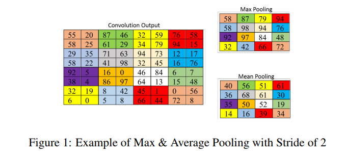
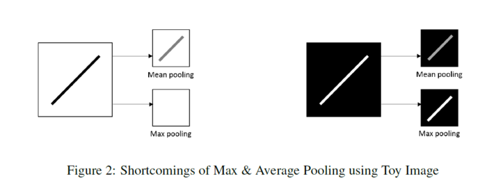
Figure 2 provides an example of the weaknesses of these two methods using toy images:
How the researchers try to combat these issues?
Using probabilistic pooling methods such as:
1. Mixed pooling: In general, when facing a new problem in which one would want to use a CNN, it is not intuitively known whether average or max-pooling should be preferred. Notably, both techniques have significant drawbacks. Average pooling forces the network to consider low magnitude (and possibly irrelevant information) in constructing representations, while max pooling can force the network to ignore fundamental differences between neighboring groups of pixels. To counteract this, mixed pooling probabilistically decides which to use during training / testing. It should be noted that, for training, it is only probabilistic in the forward pass. During back-propagation the network defaults to the earlier chosen method. Mixed pooling can be applied in 3 different ways.
- For all features within a layer
- Mixed between features within a layer
- Mixed between regions for different features within a layer
Mixed Pooling is defined as:
\begin{align} a_{kij} = \lambda \cdot max_{(p,q)\in R_{ij}}(a_{kpq})+(1-\lambda) \cdot \frac{1}{|R_{ij}|}\sum_{(p,q)\in R_{ij}}{{a_{kpq}}} \end{align}
Where [math]\displaystyle{ \lambda }[/math] is a random value 0 or 1, indicating max or average pooling for a particular region/feature/layer.
2. Stochastic pooling: improves upon max pooling by randomly sampling from neighborhood regions based on the probability values of each activation. This is defined as:
\begin{align} a_{kij} = a_l ~ \text{where } ~ l\sim P(p_1,p_2,...,p_{|R_{ij}|}) \end{align}
with probability of activations within each region defined as follows:
\begin{align} p_{pq} = \dfrac{a_{pq}}{\sum_{(p,q)} \in R_{ij} a_{pq}} \end{align}
The figure below describes the process of Stochastic Pooling. The figure on the left shows the activations of a given region, and the corresponding probability is shown in the center. The activations with the highest probability is selected by the pooling method. However, any activation can be selected. In this case, the midrange activation of 13% is selected.
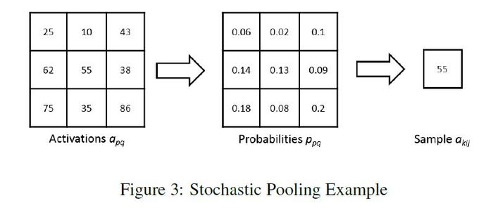
As stochastic pooling is based on probability and is not deterministic, it avoids the shortcomings of max and average pooling and enjoys some of the advantages of max pooling.
3. "Top-k activation pooling" is the method that picks the top-k activation in every pooling region. This makes sure that the maximum information can pass through subsampling gates. It is to be used with max pooling, but after max pooling, to further improve the representation capability, they pick top-k activation, sum them up, and constrain the summation by a constant. Details in this paper: https://www.hindawi.com/journals/wcmc/2018/8196906/
Wavelets and Wavelet Transform
A wavelet is a representation of a square integrable function by a certain orthonormal series generated by a wavelet. The fundamental idea of wavelet transforms is that the transformation should allow only changes in time extension, but not shape. This is affected by choosing suitable basis functions that allow for this. Changes in the time extension are expected to conform to the corresponding analysis frequency of the basis function.
The wavelet transform involves taking the inner product of a signal (in this case, the image), with these basis functions. This produces a set of coefficients for the signal. These coefficients can then be quantized and coded in order to compress the image.
One issue of note is that wavelets offer a tradeoff between resolution in frequency, or in time (or presumably, image location). For example, a sine wave will be useful to detect signals with its own frequency, but cannot detect where along the sine wave this alignment of signals is occurring. Thus, basis functions must be chosen with this tradeoff in mind.
Source: Compressing still and moving images with wavelets
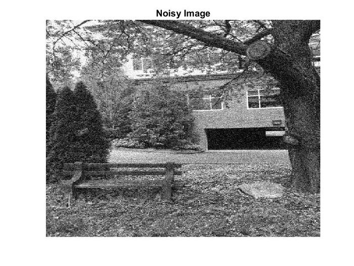
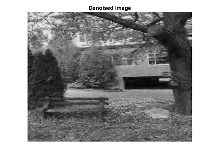
The following images show the result of applying a wavelet transform to an image for denoising:
images were taken from here.
Proposed Method
The previously highlighted pooling methods use neighborhoods to subsample, almost identical to nearest neighbor interpolation.
The proposed pooling method uses wavelets (i.e. small waves - generally used in signal processing) to reduce the dimensions of the feature maps. They use wavelet transform to minimize artifacts resulting from neighborhood reduction. They postulate that their approach, which discards the first-order sub-bands, more organically captures the data compression. The authors say that this organic reduction, therefore, lessens the creation of jagged edges and other artifacts that may impede correct image classification.
- Forward Propagation
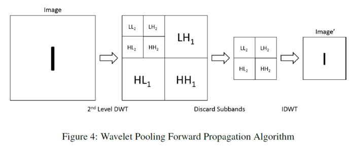
The proposed wavelet pooling scheme pools features by performing a 2nd order decomposition in the wavelet domain according to the fast wavelet transform (FWT) which is a more efficient implementation of the two-dimensional discrete wavelet transform (DWT) as follows:
\begin{align} W_{\varphi}[j+1,k] = h_{\varphi}[-n]*W_{\varphi}[j,n]|_{n=2k,k\leq0} \end{align}
\begin{align} W_{\psi}[j+1,k] = h_{\psi}[-n]*W_{\psi}[j,n]|_{n=2k,k\leq0} \end{align}
where [math]\displaystyle{ \varphi }[/math] is the approximation function, and [math]\displaystyle{ \psi }[/math] is the detail function, [math]\displaystyle{ W_{\varphi},W_{\psi} }[/math] are called approximation and detail coefficients. [math]\displaystyle{ h_{\varphi[-n]} }[/math] and [math]\displaystyle{ h_{\psi[-n]} }[/math] are the time reversed scaling and wavelet vectors, (n) represents the sample in the vector, while (j) denotes the resolution level
When using the FWT on images, it is applied twice (once on the rows, then again on the columns). By doing this in combination, the detail sub-bands (LH, HL, HH) at each decomposition level, and approximation sub-band (LL) for the highest decomposition level is obtained. After performing the 2nd order decomposition, the image features are reconstructed, but only using the 2nd order wavelet sub-bands. This method pools the image features by a factor of 2 using the inverse FWT (IFWT) which is based on the inverse DWT (IDWT).
\begin{align} W_{\varphi}[j,k] = h_{\varphi}[-n]*W_{\varphi}[j+1,n]+h_{\psi}[-n]*W_{\psi}[j+1,n]|_{n=\frac{k}{2},k\leq0} \end{align}
- Backpropagation
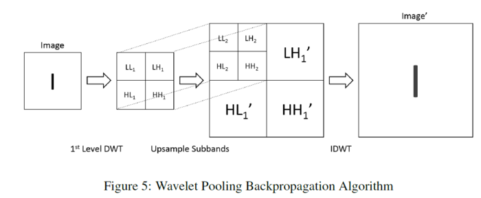
The proposed wavelet pooling algorithm performs backpropagation by reversing the process of its forward propagation. First, the image feature being backpropagated undergoes 1st order wavelet decomposition. After decomposition, the detail coefficient sub-bands up-sample by a factor of 2 to create a new 1st level decomposition. The initial decomposition then becomes the 2nd level decomposition. Finally, this new 2nd order wavelet decomposition reconstructs the image feature for further backpropagation using the IDWT. Figure 5, illustrates the wavelet pooling backpropagation algorithm in details:
Results and Discussion
All experiments have been performed using the MatConvNet(Vedaldi & Lenc, 2015) architecture. Stochastic gradient descent has been used for training. For the proposed method, the Haar wavelet has been chosen as the basis wavelet for its property of having even, square sub-bands. All CNN structures except for MNIST use a network loosely based on Zeilers network (Zeiler & Fergus, 2013). The experiments are repeated with Dropout (Srivastava, 2013) and the Local Response Normalization (Krizhevsky, 2009) is replaced with Batch Normalization (Ioffe & Szegedy, 2015) for CIFAR-10 and SHVN (Dropout only) to examine how these regularization techniques change the pooling results. The authors have tested the proposed method on four different datasets as shown in the figure:
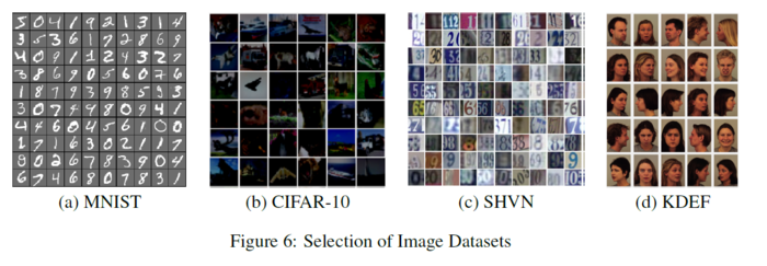
Different methods based on Max, Average, Mixed, Stochastic and Wavelet have been used at the pooling section of each architecture. Accuracy and Model Energy have been used as the metrics to evaluate the performance of the proposed methods. These have been evaluated and their performances have been compared on different data-sets.
- MNIST:
The network architecture is based on the example MNIST structure from MatConvNet, with batch-normalization, inserted. All other parameters are the same. The figure below shows their network structure for the MNIST experiments.
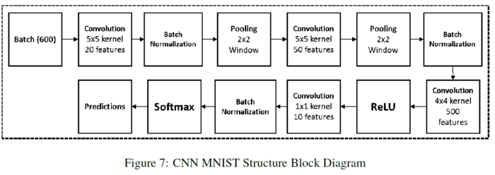
The input training data and test data come from the MNIST database of handwritten digits. The full training set of 60,000 images is used, as well as the full testing set of 10,000 images. The table below shows their proposed method outperforms all methods. Given the small number of epochs, max pooling is the only method to start to over-fit the data during training. Mixed and stochastic pooling show a rocky trajectory but do not over-fit. Average and wavelet pooling show a smoother descent in learning and error reduction. The figure below shows the energy of each method per epoch.
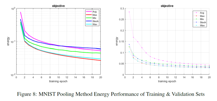
The accuracies for both paradigms are shown below:

- CIFAR-10:
The authors perform two sets of experiments with the pooling methods. The first is a regular network structure with no dropout layers. They use this network to observe each pooling method without extra regularization. The second uses dropout and batch normalization and performs over 30 more epochs to observe the effects of these changes.
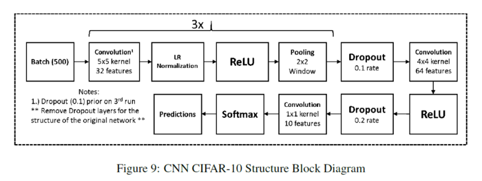
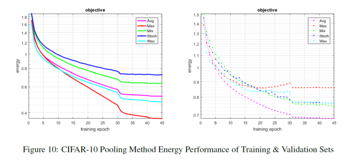
The input training and test data come from the CIFAR-10 dataset. The full training set of 50,000 images is used, as well as the full testing set of 10,000 images. For both cases, with no dropout, and with dropout, Tables below show that the proposed method has the second highest accuracy.
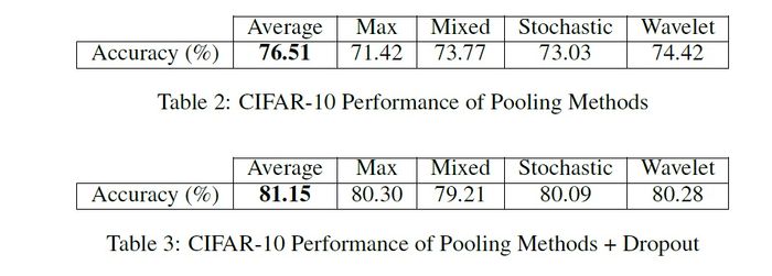
Max pooling over-fits fairly quickly, while wavelet pooling resists over-fitting. The change in learning rate prevents their method from over-fitting, and it continues to show a slower propensity for learning. Mixed and stochastic pooling maintains a consistent progression of learning, and their validation sets trend at a similar, but better rate than their proposed method. Average pooling shows the smoothest descent in learning and error reduction, especially in the validation set. The energy of each method per epoch is also shown below:
- SHVN:
Two sets of experiments are performed with the pooling methods. The first is a regular network structure with no dropout layers. They use this network to observe each pooling method without extra regularization same as what happened in the previous datasets. The second network uses dropout to observe the effects of this change. The figure below shows their network structure for the SHVN experiments:
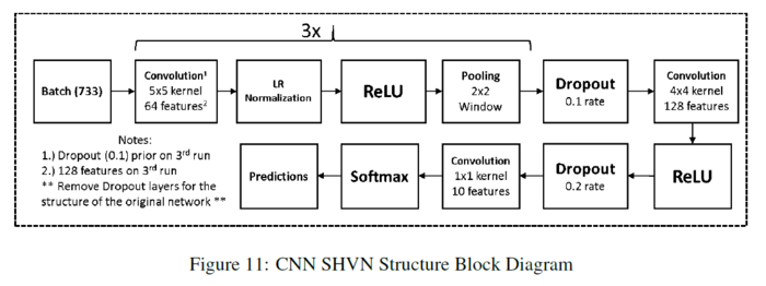
The input training and test data come from the SHVN dataset. For the case with no dropout, they use 55,000 images from the training set. For the case with dropout, they use the full training set of 73,257 images, a validation set of 30,000 images they extract from the extra training set of 531,131 images, as well as the full testing set of 26,032 images. For both cases, with no dropout, and with dropout, Tables below show their proposed method has the second lowest accuracy.
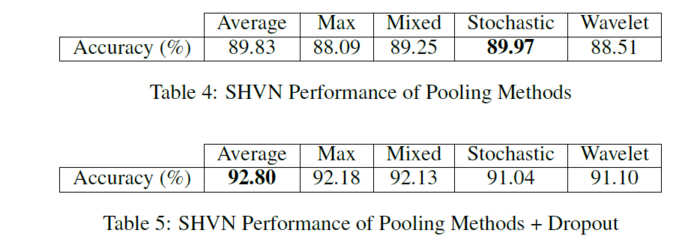
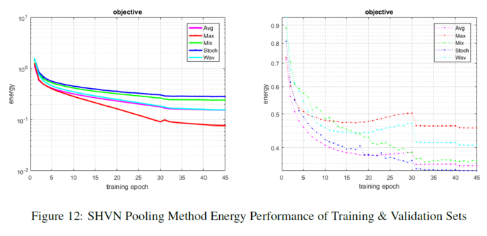
Max and wavelet pooling both slightly over-fit the data. Their method follows the path of max pooling but performs slightly better in maintaining some stability. Mixed, stochastic, and average pooling maintain a slow progression of learning, and their validation sets trend at near identical rates. The figure below shows the energy of each method per epoch.
- KDEF:
They run one set of experiments with the pooling methods that includes dropout. The figure below shows their network structure for the KDEF experiments:
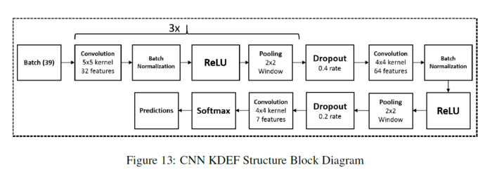
The input training and test data come from the KDEF dataset. This dataset contains 4,900 images of 35 people displaying seven basic emotions (afraid, angry, disgusted, happy, neutral, sad, and surprised) using facial expressions. They display emotions at five poses (full left and right profiles, half left and right profiles, and straight).
This dataset contains a few errors that they have fixed (missing or corrupted images, uncropped images, etc.). All of the missing images are at angles of -90, -45, 45, or 90 degrees. They fix the missing and corrupt images by mirroring their counterparts in MATLAB and adding them back to the dataset. They manually crop the images that need to match the dimensions set by the creators (762 x 562). KDEF does not designate a training or test data set. They shuffle the data and separate 3,900 images as training data, and 1,000 images as test data. They resize the images to 128x128 because of memory and time constraints.
The dropout layers regulate the network and maintain stability in spite of some pooling methods known to over-fit. The table below shows their proposed method has the second highest accuracy. Max pooling eventually over-fits, while wavelet pooling resists over-fitting. Average and mixed pooling resist over-fitting but are unstable for most of the learning. Stochastic pooling maintains a consistent progression of learning. Wavelet pooling also follows a smoother, consistent progression of learning. The figure below shows the energy of each method per epoch.
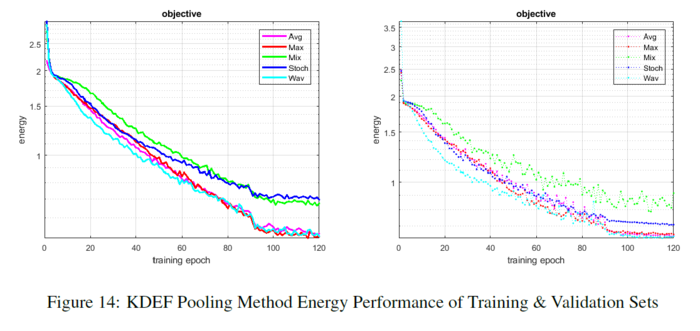
The accuracies for both paradigms are shown below:

- Computational Complexity:
Above experiments and implementations on wavelet pooling were more of a proof-of-concept rather than an optimized method. In terms of mathematical operations, the wavelet pooling method is the least computationally efficient compared to all other pooling methods mentioned above. Among all the methods, average pooling is the most efficient methods, max pooling and mix pooling are at a similar level while wavelet pooling is way more expensive to complete the calculation.
Conclusion
They prove wavelet pooling has the potential to equal or eclipse some of the traditional methods currently utilized in CNNs. Their proposed method outperforms all others in the MNIST dataset, outperforms all but one in the CIFAR-10 and KDEF datasets, and performs within respectable ranges of the pooling methods that outdo it in the SHVN dataset. The addition of dropout and batch normalization show their proposed methods response to network regularization. Like the non-dropout cases, it outperforms all but one in both the CIFAR-10 & KDEF datasets and performs within respectable ranges of the pooling methods that outdo it in the SHVN dataset.
The authors' results confirm previous studies proving that no one pooling method is superior, but some perform better than others depending on the dataset and network structure Boureau et al. (2010); Lee et al. (2016). Furthermore, many networks alternate between different pooling methods to maximize the effectiveness of each method. [1]
Future work and improvements in this area could be to vary the wavelet basis to explore which basis performs best for the pooling. Altering the upsampling and downsampling factors in the decomposition and reconstruction can lead to better image feature reductions outside of the 2x2 scale. Retention of the subbands we discard for the backpropagation could lead to higher accuracies and fewer errors. Improving the method of FTW we use could greatly increase computational efficiency. Finally, analyzing the structural similarity (SSIM) of wavelet pooling versus other methods could further prove the vitality of using the authors' approach. [1]
Suggested Future work
Upsampling and downsampling factors in decomposition and reconstruction need to be changed to achieve more feature reduction. The subbands that we previously discard should be kept for higher accuracies. To achieve higher computational efficiency, improving the FTW method is needed.
Critiques and Suggestions
- The functionality of backpropagation process which can be a positive point of the study is not described enough comparing to the existing methods.
- The main study is on wavelet decomposition while the reason of using Haar as mother wavelet and the number of decomposition levels selection has not been described and are just mentioned as a future study!
- At the beginning, the study mentions that the pooling method is not under attention as it should be. In the end, results show that choosing the pooling method depends on the dataset and they mention trial and test as a reasonable approach to choose the pooling method. In my point of view, the authors have not really been focused on providing a pooling method which can help the current conditions to be improved effectively. At least, trying to extract a better pattern for relating results to the dataset structure could be so helpful.
- Average pooling origins which are mentioned as the main pooling algorithm to compare with, is not even referenced in the introduction.
- Combination of the wavelet, Max and Average pooling can be an interesting option to investigate more on this topic; both in a row(Max/Avg after wavelet pooling) and combined like mix pooling option.
- While the current datasets express the performance of the proposed method in an appropriate way, it could be a good idea to evaluate the method using some larger datasets. Maybe it helps to understand whether the size of a dataset can affect the overfitting behavior of max pooling which is mentioned in the paper.
- Adding asymptotic notations to the computational complexity of the proposed algorithm would be meaningful, particularly since the given results are for a single/fixed input size (one image in forward propagation) and consequently are not generalizable.
- They could have considered comparing against Fast Fourier Transform (FFT). Including a non-wavelet form seems to be an obvious candidate for comparison
- If they went beyond the 2x2 pooling window this would have further supported their method
- ([[1]]) The experiments are largely conducted with very small scale datasets. As a result, I am not sure if they are representative enough to show the performance difference between different pooling methods.
- ([[2]]) No comparison to non-wavelet methods. For example, one obvious comparison would have been to look at using a DCT or FFT transform where the output would discard high-frequency components (this can get very close to the wavelet idea!). Also, this critique might provides us with some interesting research directions since DCT or FFT transforms as pooling are not throughly studied yet.
- Also, convolutional neural network are not only used in image related tasks. Evaluating the efficiency of wavelet pooling in convolutional neural network applied to natural languages or other applicable areas will be interesting. Such experiments shall also show if such approach can be generalized.
References
Williams, Travis, and Robert Li. "Wavelet Pooling for Convolutional Neural Networks." (2018).
Hilton, Michael L., Björn D. Jawerth, and Ayan Sengupta. "Compressing still and moving images with wavelets." Multimedia systems 2.5 (1994): 218-227.
Revisions
- Two reviewers really liked the paper and one of them called it in the top 15% papers in the conference which supports the novelty and potential of the idea. One other reviewer, however, believed that this was not good enough to be accepted and the main reason for rejection was the linearity nature of wavelet(which was not convincingly described).
- The main concern of two of the reviewers has been the size of the datasets that have been used to test the method and the authors have mentioned future works concerning bigger datasets to test the method.
- The computational cost section had not been included in the paper initially and was added after one of the reviewer's concern. So, the other reviewers have not been curious about this and unfortunately, there is no comment on that from them. However, the description on the non-efficient implementation seemed to be satisfactory to the reviewer which resulted in being accepted.
At the end, if you are interested in implementing the method, they are willing to share their code but after making it efficient. So, maybe there will be another paper regarding less computational cost on larger datasets with a publishable code.
