Annotating Object Instances with a Polygon RNN: Difference between revisions
m (Added results section) |
|||
| (61 intermediate revisions by 21 users not shown) | |||
| Line 1: | Line 1: | ||
Summary of the CVPR '17 best [https://www.cs.utoronto.ca/~fidler/papers/paper_polyrnn.pdf ''paper''] | Summary of the CVPR '17 best [https://www.cs.utoronto.ca/~fidler/papers/paper_polyrnn.pdf ''paper''] | ||
= | The presentation video of paper is available here[https://www.youtube.com/watch?v=S1UUR4FlJ84]. | ||
= Background = | |||
If a snapshot of an image is given to a human, how will he/she describe a scene? He/she might identify that there is a car parked near the curb, or that the car is parked right beside a street light. This ability to decompose objects in scenes into separate entities is key to understanding what is around us and it helps to reason about the behavior of objects in the scene. | |||
Automating this process is a classic computer vision problem and is often termed "object detection". There are four distinct levels of detection (refer to Figure 1 for a visual cue): | |||
2. Object Detection: The classic definition of object detection points to the detection and localization of '''multiple''' objects of interest in the image. The output of the detection is still a bounding box overlayed on the image at the position corresponding the location of the objects in the image. | 1. Classification + Localization: This is the most basic method that detects whether '''an''' object is either present or absent in the image and then identifies the position of the object within the image in the form of a bounding box overlayed on the image. | ||
2. Object Detection: The classic definition of object detection points to the detection and localization of '''multiple''' objects of interest in the image. The output of the detection is still a bounding box overlayed on the image at the position corresponding to the location of the objects in the image. | |||
3. Semantic Segmentation: This is a pixel level approach, i.e., each pixel in the image is assigned to a category label. Here, there is no difference between instances; this is to say that there are objects present from three distinct categories in the image, without tracking or reporting the number of appearances of each instance within a category. | 3. Semantic Segmentation: This is a pixel level approach, i.e., each pixel in the image is assigned to a category label. Here, there is no difference between instances; this is to say that there are objects present from three distinct categories in the image, without tracking or reporting the number of appearances of each instance within a category. | ||
4. Instance Segmentation: The goal | 4. Instance Segmentation (''This paper performs this''): The goal is to not only to assign pixel-level categorical labels, but to identify each entity separately as sheep 1, sheep 2, sheep 3, grass, and so on. | ||
[[File:Figure_1.jpeg | 450px|thumb|center|Figure 1: Different levels of detection in an image.]] | [[File:Figure_1.jpeg | 450px|thumb|center|Figure 1: Different levels of detection in an image.]] | ||
| Line 20: | Line 22: | ||
== Motivation == | == Motivation == | ||
Semantic segmentation helps us achieve a deeper understanding of images than image classification or object detection. Over and above this, instance segmentation is crucial | Semantic segmentation helps us achieve a deeper understanding of images than image classification or object detection. Over and above this, instance segmentation is crucial in applications where multiple objects of the same category are to be tracked, especially in autonomous driving, mobile robotics, and medical image processing. This paper deals with a novel method to tackle the instance segmentation problem pertaining specifically to the field of autonomous driving, but shown to generalize well in other fields such as medical image processing. | ||
A polygon is natural form of annotation. Current instant segmentations annotated by humans use polygons because it is a special representation of the image which can use small number of vertices instead of various pixels and makes it easy to incorporate user modifications. | |||
[[File:polygon.png|600px|center]] | |||
== Goal == | |||
Most of the recent approaches to on instance segmentation are based on deep neural networks and have demonstrated impressive performance. Given that these approaches require a lot of computational resources and that their performance depends on the amount of accessible training data, there has been an increase in the demand to label/annotate large-scale datasets. This is both expensive and time-consuming. | |||
{| class=wikitable width=700 align=center | |||
|Thus, the '''main goal''' of the paper is to enable '''semi-automatic''' annotation of object instances. | |||
|} | |||
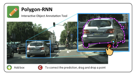
Figure 2 demonstrates how the interface looks like for better clarity. | |||
Most of the datasets available pass through a stage where annotators manually outline the objects with a closed polygon. Polygons allow annotation of objects with a small number of clicks (30 - 40) compared to other methods. This approach works as the silhouette of an object is typically connected without holes. | |||
{| class=wikitable width=900 align=center | |||
|Thus, the authors suggest to adopt this same technique to annotate images using polygons, except they plan to automate the method and replace/reduce manual labeling. The '''intuition''' behind the success of this method is the '''sparse''' nature of these polygons that allow annotating of an object through a cluster of pixels rather than classification at the pixel level. | |||
|} | |||
[[File:Annotating Object Instances Example.png | 450px|thumb|center|Figure 2: Given a bounding box, polygon outlining the object instance inside the box is predicted. This approach is designed to facilitation annotation, and easily incorporates user corrections of points to improve the overall object’s polygon. ]] | |||
= Related Works = | |||
Some of the techniques used in semi-automatic annotation are as follows: | |||
1. '''GrabCut''': In general, GrabCut is a method to separate the foreground and background of an image with minimal user interaction. Specifically, the user needs to only create a rectangular bounding box containing the foreground, and the algorithm will extract the object in the foreground. A major contribution of the paper is that labeling (of the object in the foreground) was not required, as the algorithm was able to identify where significant changes in colour pattern occurred. In this sense, it mimics automatic segmentation when combined with a Region Proposal Network. | |||
[[File:GrabCut_Example.png | 450px|thumb|center|Figure 3: Illustration of GrabCut.]] | |||
2. '''GrabCut + CNN''': Scribbles have also been used to train CNNs for semantic image segmentation. | |||
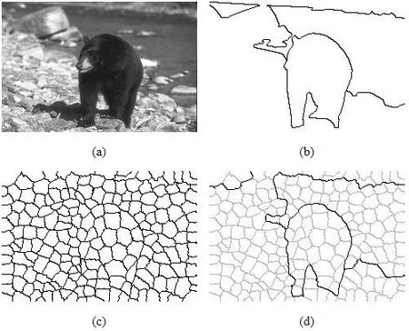
3. '''Superpixels''': Superpixels in the form of small polygons where the color intensity within each superpixel is similar, to a certain threshold, have been used to provide a sparse representation of large number of pixels in an image. However, the performance of this technique depends on the scale of the superpixels and hence sometimes merges small objects. | |||
[[File:Superpixel_idea.jpg | 450px|thumb|center|Figure 4: Illustration of the superpixel idea.]] | |||
= Model = | = Model = | ||
As an input to | As an '''input''' to the model, an annotator or perhaps another neural network provides a bounding box containing an object of interest and the model auto-generates a polygon outlining the object instance using a Recurrent Neural Network which they call: Polygon-RNN. | ||
The RNN model predicts | The RNN model predicts the vertices of the polygon at each time step given a CNN representation of the image, the last two time steps, and the first vertex location. The location of the first vertex is defined differently and will be defined shortly. The information regarding the previous two-time steps helps the RNN create a polygon in a specific direction and the first vertex provides a cue for loop closure of the polygon edges. | ||
The polygon is parametrized as a sequence of 2D vertices and it is assumed that the polygon is closed. In addition, the polygon generation is fixed to follow a clockwise orientation since there are multiple ways to create a polygon given that it is cyclic structure. However, the starting point of the sequence is defined so that it can be any of the vertices of the polygon. | The polygon is parametrized as a sequence of 2D vertices and it is assumed that the polygon is closed. In addition, the polygon generation is fixed to follow a clockwise orientation since there are multiple ways to create a polygon given that it is cyclic structure. However, the starting point of the sequence is defined so that it can be any of the vertices of the polygon. | ||
| Line 38: | Line 72: | ||
There are two primary networks at play: 1. CNN with skip connections, and 2. One-to-many type RNN. | There are two primary networks at play: 1. CNN with skip connections, and 2. One-to-many type RNN. | ||
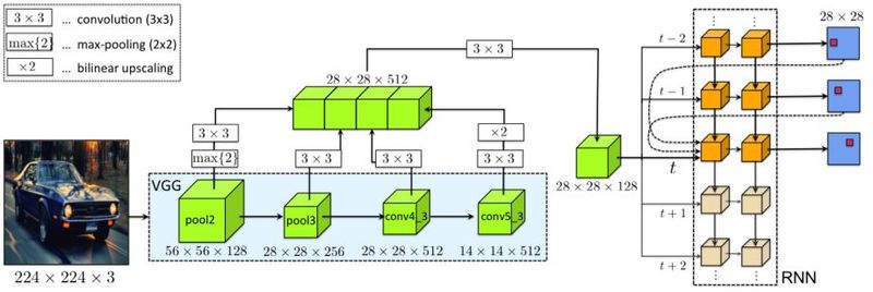
[[File:Figure_2_Neel.JPG | 800px|thumb|center|Figure | [[File:Figure_2_Neel.JPG | 800px|thumb|center|Figure 5: Model architecture for Polygon-RNN depicting a CNN with skip connections feeding into a 2 layer ConvLSTM (One-to-many type) ('''Note''': A possible point of confusion - the authors have only shown the layers of VGG16 architecture here that have the skip connections introduced).]] | ||
1. '''CNN with skip connections''': | 1. '''CNN with skip connections''': | ||
The authors have adopted the VGG16 feature extractor architecture with a few modifications pertaining to preservation of | The authors have adopted the VGG16 feature extractor architecture with a few modifications pertaining to the preservation of features fused together in a tensor that can feed into the RNN (refer to Figure 5). Namely, the last max-pooling layer (''pool5'') present in the VGG16 CNN has been removed. The image fed into the CNN is pre-shrunk to a 224x224x3 tensor(3 being the Red, Green, and Blue channels). The image passes through 2 pooling layers and 2 convolutional layers. Since, the features extracted after each operation are to be preserved and fused later on, at each of these four steps, the idea is to have a tensor with a common width of 512; so the output tensor at pool2 is convolved with 4 3x3x128 filters and the output tensor at pool3 is convolved with 2 3x3x256 filters. The skip connections from the four layers allow the CNN to extract low-level edge and corner features (helps to follow the object's boundaries) as well as boundary/semantic information about the instances (helps to identify the object). Finally, a 3x3 convolution applied along with a ReLU non-linearity results in a 28x28x128 tensor that contains semantic information pertinent to the image frame and is taken as an input by the RNN. | ||
2. '''RNN - 2 Layer ConvLSTM''' | 2. '''RNN - 2 Layer ConvLSTM''' | ||
The RNN is employed to capture information about the previous vertices in the time-series. Specifically, a Convolutional LSTM is used as a decoder. The ConvLSTM allows preservation of the spatial information in 2D and reduces the number of parameters compared to a Fully Connected RNN. The polygon is modeled with a kernel size of 3x3 and 16 channels outputting a vertex at each time step. | The RNN is employed to capture information about the previous vertices in the time-series. Specifically, a Convolutional LSTM is used as a decoder. The ConvLSTM allows preservation of the spatial information in 2D received from CNN and reduces the number of parameters compared to a Fully Connected RNN. The polygon is modeled with a kernel size of 3x3 and 16 channels outputting a vertex at each time step. The ConvLSTM gets as input a tensor step t which | ||
concatenates 4 features: the CNN feature representation of the image, one-hot encoding of the previously predicted vertex and the vertex predicted | |||
from two-time steps ago, as well as the one-hot encoding of the first predicted vertex. | |||
The Convolutional LSTM computes the hidden state <math display = "inline">h_t</math> given the input <math display = "inline">x_t</math> based on the following equations: | |||
<center> | |||
<math display="block"> | |||
\begin{pmatrix} | |||
i_t \\ | |||
f_t \\ | |||
o_t \\ | |||
g_t \\ | |||
\end{pmatrix} | |||
= W_h * h_{t-1} + W_x * x_t + b | |||
</math> | |||
<math display="block"> | |||
c_t = \sigma(f_t) \bigodot c_{t-1} + \sigma(i_t) \bigodot tanh(g_t) | |||
</math> | |||
<math display="block"> | |||
h_t = \sigma(o_t) \bigodot tanh(c_t) | |||
</math> | |||
</center> | |||
where <math display = "inline">i, f, o</math> denote the input, forget, and output gate, <math display = "inline">h</math> is the hidden state and <math display = "inline">c</math> is the cell state. Also, <math display = "inline">\sigma</math> denotes the sigmoid function, <math display = "inline">\bigodot</math> indicates an element-wise product and <math display = "inline">*</math> a convolution. <math display = "inline">W_h</math> denotes the hidden-to-state convolution kernel and <math display = "inline">W_x</math> the input-to-state convolution kernel. | |||
The authors have treated the vertex prediction task as a classification task in that the location of the vertices is through a one-hot representation of dimension DxD + 1 (D chosen to be 28 by the authors in tests). The one | The authors have treated the vertex prediction task as a classification task in that the location of the vertices is through a one-hot representation of dimension DxD + 1 (D chosen to be 28 by the authors in tests). The one additional dimension is the storage cue for loop closure for the polygon. Given that, the one-hot representation of the two previously predicted vertices and the first vertex are taken in as an input, a clockwise (or for that reason any fixed direction) direction can be forced for the creation of the polygon. Coming back to the prediction of the first vertex, as polygon is a circle, any vertex of a polygon can be used as a starting point. Therefore the authors treat the starting point as special, and this is done through further modification of the CNN by adding two DxD layers with one branch predicting object instance boundaries while the other takes in this output as well as the image features to predict vertices of the polygon. The boundaries and vertices prediction are being treated as binary classification problem in each cell in the output grid. This CNN is trained separately. Here, <math display = "inline">y_t</math> denotes the one-hot encoding of the vertex and is the output at time step <math>t</math>. | ||
== Training == | == Training == | ||
| Line 54: | Line 112: | ||
The training of the model is done as follows: | The training of the model is done as follows: | ||
1. Cross entropy is used for the RNN | 1. Cross-entropy is used for the RNN loss function. To avoid over-penalizing of mispredictions that are close to the ground-truth vertex, non-zero probability mass is assigned to locations which are within a distance of 2 in D × D output grid. | ||
2. Instead of Stochastic Gradient Descent, Adam is used for optimization: batch size = 8, learning rate = 1e^-4 (learning rate decays after 10 epochs by a factor of 10) | |||
3. For the first vertex prediction, the modified CNN | 2. The typical training regime, where the model make predictions at each time step but feed in ground-truth vertex information to the next, is followed. Instead of Stochastic Gradient Descent, Adam is used for optimization: batch size = 8, learning rate = 1e^-4 (learning rate decays after 10 epochs by a factor of 10) This choice of optimizer makes it easier for development, but switching back to SGD may get better experimental results due to convergence problems of Adam. | ||
3. For the first vertex prediction, the modified CNN mentioned previously, is trained using a multi-task cost function. In particular, the authors used the logistic loss for every location in the grid. | |||
The reported time for training is one day on a Nvidia Titan-X GPU. | The reported time for training is one day on a Nvidia Titan-X GPU. | ||
== | The resolution of the polygon is 28 x 28, based on the downsampling factor and ConvLSTM resolution. They simplified the polygon by removing vertices on the grid line and the same vertices that fall in the same grid. They also randomly flipped images, enlarged original bounding boxes and randomly selected the starting vertex of the polygon notation as their data augmentation process. | ||
== Importance of Human Annotator in the Loop == | |||
The model allows for the prediction at a given time step to be corrected and this corrected vertex is then fed into the next time step of the RNN, effectively rejecting the network predicted vertex. This has the simple effect of putting the model "back on the right track". Note that this is only possible due to the adoption of the RNN architecture i.e. the inherent nature of the RNN to accept previous outputs allows incorporation of the user's judgement. The typical inference time as quoted by the paper is 250ms per object. | |||
In addition, the role of the human annotator also serves to evaluate quantitatively the suggested approach, both in terms of accuracy as well as tracing time. The Cityscapes dataset was used to obtain a number of validation images segmented by the human annotator and the semi-automatic algorithm. However, the evaluation process also raises some questions about the objectivity of the current object-segmentation metrics considering that ground-truth pixel-segmented images are both traced and evaluated by human annotators. Despite the minor percentage of error in the semi-automatic approach, it achieves a remarkable performance in terms of tracing time in comparison with all the available benchmarks. | |||
= Results = | |||
== Evaluation Metrics == | |||
The evaluation of the model performance was conducted based on the Cityscapes and KITTI Datasets. There are two metrics used for evaluation: | |||
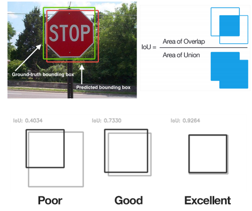
1. '''IoU''': The standard Intersection over Union (IoU) measure is used for comparison. In add The calculation for IoU takes both the predicted and ground-truth object boundaries. The intersection (area contained in both boundaries at once) is divided by the union (the area contained by at least one, or both, of the boundaries). A low score of this metric would mean that there is little overlap between the boundaries, or large areas on non-overlap, and a score of 1.0 would indicate that the two boundaries contain the same area. | |||
An example of the IoU is illustrated in the figure below: | |||
[[File:IoU_figure.png|500px|center]] Source:https://www.pyimagesearch.com/2016/11/07/intersection-over-union-iou-for-object-detection/ | |||
2. '''Number of Clicks''': To evaluate the speed up factor, the checkerboard distance is used to measure the distance between the ground truth (GT) and the output of the Polygon RNN. A set of distance thresholds are set <math display = "inline">T ∈ [1,2,3,4]</math> and if the distance exceeds the particular threshold, the correction is made by an annotator to match the GT and the '''Number of Clicks''' is used to evaluate the speed up factor. | |||
== Baseline Techniques == | |||
1. '''SharpMask''': a 50 layer ResNet considered as the state of the art annotation method. | |||
2. '''DeepMask''': a build-up on the 50 layer ResNet with an addition of another CNN. | |||
3. '''Dilation10''': another simple technique using purely convolutional operations. | |||
4. '''SquareBox''': a simple technique where an entire bounding box is labeled as an object | |||
== Quantitative Results == | |||
We report the IoU metric in Table | |||
1. The Polygon RNN method outperforms the baselines in 6 out of the 8 categories and has a mean IoU greater than all of the baselines. Particularly, in the car, person, and rider categories, a 12%, 7%, and 6% higher performance than SharpMask is achieved. | |||
[[File:Table_1_Neel.JPG | 800px|thumb|center|Table 1: IoU performance on Cityscapes data without any annotator intervention.]] | |||
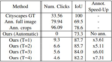
In addition, with the help of the annotator, the speedup factor was 7.3 times with under 5 clicks which the authors claim is the main advantage of this method. | |||
[[File:Table_0_Neel.JPG | 800px|thumb|center|Table 2: IoU performance on Cityscapes data with annotator intervention.]] | |||
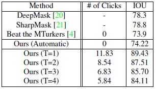
The method also works well with other datasets such as KITTI: | |||
[[File:Table_2_Neel.JPG | 800px|thumb|center|Table 3: IoU performance on KITTI data.]] | |||
== Effect of object size == | |||
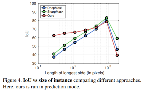
In Fig. 4, we see how our model performs w.r.t baselines on different instance sizes. For small instances, our model performs significantly better than the baselines. For larger objects, the baselines have an advantage due to the larger output resolution. | |||
[[File:IoU_vs_size_of_instance.PNG | 500px|thumb|center|Fig 4: IoU_vs_size_of_instance.]] | |||
== Qualitative Results == | |||
In addition, most of the comparisons with human annotators show that the method is at par with human-level annotation. | |||
<gallery widths=500px heights=500px perrow=2 mode="packed"> | |||
File:Figure_3_Neel.JPG|Figure 6: Qualitative results: comparison with human annotator.|alt=alt language | |||
File:Figure_4_Neel.JPG|Figure 7: Qualitative results: comparison with human annotator.|alt=alt language | |||
</gallery> | |||
=Conclusion= | |||
The important conclusions from this paper are: | |||
1. The paper presented a powerful generic annotation tool for modelling complex annotations as a simple polygon that works on different unseen datasets. | |||
2. Significant improvement in annotation time can be achieved with the Polygon-RNN method itself (speed-up factor of 4.74). | |||
3. However, the flexibility of having inputs from a human annotator helps increase the IoU for a certain range of clicks. | |||
4. The model architecture has a down-sampling factor of 16 and the final output resolution and accuracy is sensitive to object size. | |||
5. Another downside of the model architecture is that training time is increased due to the training of the CNN for the first vertex. | |||
=Critique= | |||
1. With the human annotator in the loop, the model speeds up the process of annotation by over 7 times which is perhaps a big cost and time cutting improvement for companies. | |||
2. Given that this model uses the VGG16 architecture compared to the 50 layer ResNet in SharpMask, this method is quite efficient. | |||
3. This paper requires training of an entire CNN for the first vertex and is inefficient in that sense as it introduces additional parameters adding to the computation time and resource demand. | |||
4. The baseline methods have an upper hand compared to this model when it comes to larger objects since the nature of the down-scaled structure adopted by this model. | |||
5. In terms of future work, elimination of the additional CNN for the first vertex as well as an enhanced architecture to remain insensitive to the size of the object to be annotated should be implemented. | |||
6. Compared to other models, the model was shown to not perform as well for larger objects (see table 3). This is likely due to the fact that vertex location determination is done in a highly compressed (28x28) representation compared to the input image(224x224). For larger objects, bounding boxes are larger. Each vertex represents many pixels. When up-converted back to the input image/bounding box size these may lead to errors especially when considering a very precise evaluation metric (intersection over union) is used. Potentially, the results can be improved by considering a higher resolution for the internal representation or one that scales with the size of the bounding. | |||
7. While the model outperforms the baseline for certain categories of object, it is surprising that it underperforms in categories such as 'bus' and 'train'. With human annotators in the loop, one would expect the model to outperform in all categories. | |||
8. One of the major contributions of this paper lies on the fact that this paper presents a method that does have an applicable value in the real world. In the paper, it does show that it can greatly reduce the human labeling efforts, and with human collaboration, this algorithm can help us tackle the image labeling problem much more efficiently. However, it does not provide the theoretical explanation that why would an RNN work better than a CNN in this case, a more in-depth analysis would make the paper better. | |||
=Code= | |||
# [https://github.com/AlexMa011/pytorch-polygon-rnn] (unofficial) | |||
# Code for an updated version of the model is available at [https://github.com/fidler-lab/polyrnn-pp] (official) | |||
Latest revision as of 18:41, 16 December 2018
Summary of the CVPR '17 best paper
The presentation video of paper is available here[1].
Background
If a snapshot of an image is given to a human, how will he/she describe a scene? He/she might identify that there is a car parked near the curb, or that the car is parked right beside a street light. This ability to decompose objects in scenes into separate entities is key to understanding what is around us and it helps to reason about the behavior of objects in the scene.
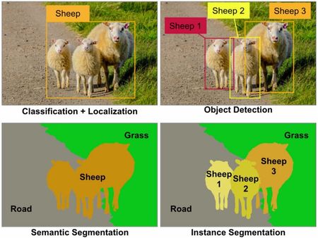
Automating this process is a classic computer vision problem and is often termed "object detection". There are four distinct levels of detection (refer to Figure 1 for a visual cue):
1. Classification + Localization: This is the most basic method that detects whether an object is either present or absent in the image and then identifies the position of the object within the image in the form of a bounding box overlayed on the image.
2. Object Detection: The classic definition of object detection points to the detection and localization of multiple objects of interest in the image. The output of the detection is still a bounding box overlayed on the image at the position corresponding to the location of the objects in the image.
3. Semantic Segmentation: This is a pixel level approach, i.e., each pixel in the image is assigned to a category label. Here, there is no difference between instances; this is to say that there are objects present from three distinct categories in the image, without tracking or reporting the number of appearances of each instance within a category.
4. Instance Segmentation (This paper performs this): The goal is to not only to assign pixel-level categorical labels, but to identify each entity separately as sheep 1, sheep 2, sheep 3, grass, and so on.
Motivation
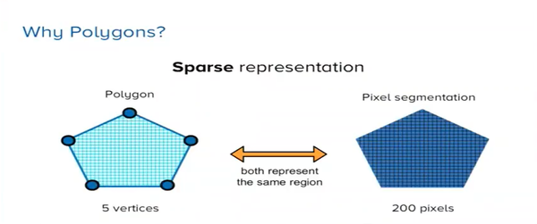
Semantic segmentation helps us achieve a deeper understanding of images than image classification or object detection. Over and above this, instance segmentation is crucial in applications where multiple objects of the same category are to be tracked, especially in autonomous driving, mobile robotics, and medical image processing. This paper deals with a novel method to tackle the instance segmentation problem pertaining specifically to the field of autonomous driving, but shown to generalize well in other fields such as medical image processing. A polygon is natural form of annotation. Current instant segmentations annotated by humans use polygons because it is a special representation of the image which can use small number of vertices instead of various pixels and makes it easy to incorporate user modifications.
Goal
Most of the recent approaches to on instance segmentation are based on deep neural networks and have demonstrated impressive performance. Given that these approaches require a lot of computational resources and that their performance depends on the amount of accessible training data, there has been an increase in the demand to label/annotate large-scale datasets. This is both expensive and time-consuming.
| Thus, the main goal of the paper is to enable semi-automatic annotation of object instances. |
Figure 2 demonstrates how the interface looks like for better clarity.
Most of the datasets available pass through a stage where annotators manually outline the objects with a closed polygon. Polygons allow annotation of objects with a small number of clicks (30 - 40) compared to other methods. This approach works as the silhouette of an object is typically connected without holes.
| Thus, the authors suggest to adopt this same technique to annotate images using polygons, except they plan to automate the method and replace/reduce manual labeling. The intuition behind the success of this method is the sparse nature of these polygons that allow annotating of an object through a cluster of pixels rather than classification at the pixel level. |
Related Works
Some of the techniques used in semi-automatic annotation are as follows:
1. GrabCut: In general, GrabCut is a method to separate the foreground and background of an image with minimal user interaction. Specifically, the user needs to only create a rectangular bounding box containing the foreground, and the algorithm will extract the object in the foreground. A major contribution of the paper is that labeling (of the object in the foreground) was not required, as the algorithm was able to identify where significant changes in colour pattern occurred. In this sense, it mimics automatic segmentation when combined with a Region Proposal Network.

2. GrabCut + CNN: Scribbles have also been used to train CNNs for semantic image segmentation.
3. Superpixels: Superpixels in the form of small polygons where the color intensity within each superpixel is similar, to a certain threshold, have been used to provide a sparse representation of large number of pixels in an image. However, the performance of this technique depends on the scale of the superpixels and hence sometimes merges small objects.
Model
As an input to the model, an annotator or perhaps another neural network provides a bounding box containing an object of interest and the model auto-generates a polygon outlining the object instance using a Recurrent Neural Network which they call: Polygon-RNN.
The RNN model predicts the vertices of the polygon at each time step given a CNN representation of the image, the last two time steps, and the first vertex location. The location of the first vertex is defined differently and will be defined shortly. The information regarding the previous two-time steps helps the RNN create a polygon in a specific direction and the first vertex provides a cue for loop closure of the polygon edges.
The polygon is parametrized as a sequence of 2D vertices and it is assumed that the polygon is closed. In addition, the polygon generation is fixed to follow a clockwise orientation since there are multiple ways to create a polygon given that it is cyclic structure. However, the starting point of the sequence is defined so that it can be any of the vertices of the polygon.
Architecture
There are two primary networks at play: 1. CNN with skip connections, and 2. One-to-many type RNN.
1. CNN with skip connections:
The authors have adopted the VGG16 feature extractor architecture with a few modifications pertaining to the preservation of features fused together in a tensor that can feed into the RNN (refer to Figure 5). Namely, the last max-pooling layer (pool5) present in the VGG16 CNN has been removed. The image fed into the CNN is pre-shrunk to a 224x224x3 tensor(3 being the Red, Green, and Blue channels). The image passes through 2 pooling layers and 2 convolutional layers. Since, the features extracted after each operation are to be preserved and fused later on, at each of these four steps, the idea is to have a tensor with a common width of 512; so the output tensor at pool2 is convolved with 4 3x3x128 filters and the output tensor at pool3 is convolved with 2 3x3x256 filters. The skip connections from the four layers allow the CNN to extract low-level edge and corner features (helps to follow the object's boundaries) as well as boundary/semantic information about the instances (helps to identify the object). Finally, a 3x3 convolution applied along with a ReLU non-linearity results in a 28x28x128 tensor that contains semantic information pertinent to the image frame and is taken as an input by the RNN.
2. RNN - 2 Layer ConvLSTM
The RNN is employed to capture information about the previous vertices in the time-series. Specifically, a Convolutional LSTM is used as a decoder. The ConvLSTM allows preservation of the spatial information in 2D received from CNN and reduces the number of parameters compared to a Fully Connected RNN. The polygon is modeled with a kernel size of 3x3 and 16 channels outputting a vertex at each time step. The ConvLSTM gets as input a tensor step t which concatenates 4 features: the CNN feature representation of the image, one-hot encoding of the previously predicted vertex and the vertex predicted from two-time steps ago, as well as the one-hot encoding of the first predicted vertex.
The Convolutional LSTM computes the hidden state [math]\displaystyle{ h_t }[/math] given the input [math]\displaystyle{ x_t }[/math] based on the following equations:
[math]\displaystyle{ \begin{pmatrix} i_t \\ f_t \\ o_t \\ g_t \\ \end{pmatrix} = W_h * h_{t-1} + W_x * x_t + b }[/math]
[math]\displaystyle{ c_t = \sigma(f_t) \bigodot c_{t-1} + \sigma(i_t) \bigodot tanh(g_t) }[/math]
[math]\displaystyle{ h_t = \sigma(o_t) \bigodot tanh(c_t) }[/math]
where [math]\displaystyle{ i, f, o }[/math] denote the input, forget, and output gate, [math]\displaystyle{ h }[/math] is the hidden state and [math]\displaystyle{ c }[/math] is the cell state. Also, [math]\displaystyle{ \sigma }[/math] denotes the sigmoid function, [math]\displaystyle{ \bigodot }[/math] indicates an element-wise product and [math]\displaystyle{ * }[/math] a convolution. [math]\displaystyle{ W_h }[/math] denotes the hidden-to-state convolution kernel and [math]\displaystyle{ W_x }[/math] the input-to-state convolution kernel.
The authors have treated the vertex prediction task as a classification task in that the location of the vertices is through a one-hot representation of dimension DxD + 1 (D chosen to be 28 by the authors in tests). The one additional dimension is the storage cue for loop closure for the polygon. Given that, the one-hot representation of the two previously predicted vertices and the first vertex are taken in as an input, a clockwise (or for that reason any fixed direction) direction can be forced for the creation of the polygon. Coming back to the prediction of the first vertex, as polygon is a circle, any vertex of a polygon can be used as a starting point. Therefore the authors treat the starting point as special, and this is done through further modification of the CNN by adding two DxD layers with one branch predicting object instance boundaries while the other takes in this output as well as the image features to predict vertices of the polygon. The boundaries and vertices prediction are being treated as binary classification problem in each cell in the output grid. This CNN is trained separately. Here, [math]\displaystyle{ y_t }[/math] denotes the one-hot encoding of the vertex and is the output at time step [math]\displaystyle{ t }[/math].
Training
The training of the model is done as follows:
1. Cross-entropy is used for the RNN loss function. To avoid over-penalizing of mispredictions that are close to the ground-truth vertex, non-zero probability mass is assigned to locations which are within a distance of 2 in D × D output grid.
2. The typical training regime, where the model make predictions at each time step but feed in ground-truth vertex information to the next, is followed. Instead of Stochastic Gradient Descent, Adam is used for optimization: batch size = 8, learning rate = 1e^-4 (learning rate decays after 10 epochs by a factor of 10) This choice of optimizer makes it easier for development, but switching back to SGD may get better experimental results due to convergence problems of Adam.
3. For the first vertex prediction, the modified CNN mentioned previously, is trained using a multi-task cost function. In particular, the authors used the logistic loss for every location in the grid.
The reported time for training is one day on a Nvidia Titan-X GPU.
The resolution of the polygon is 28 x 28, based on the downsampling factor and ConvLSTM resolution. They simplified the polygon by removing vertices on the grid line and the same vertices that fall in the same grid. They also randomly flipped images, enlarged original bounding boxes and randomly selected the starting vertex of the polygon notation as their data augmentation process.
Importance of Human Annotator in the Loop
The model allows for the prediction at a given time step to be corrected and this corrected vertex is then fed into the next time step of the RNN, effectively rejecting the network predicted vertex. This has the simple effect of putting the model "back on the right track". Note that this is only possible due to the adoption of the RNN architecture i.e. the inherent nature of the RNN to accept previous outputs allows incorporation of the user's judgement. The typical inference time as quoted by the paper is 250ms per object.
In addition, the role of the human annotator also serves to evaluate quantitatively the suggested approach, both in terms of accuracy as well as tracing time. The Cityscapes dataset was used to obtain a number of validation images segmented by the human annotator and the semi-automatic algorithm. However, the evaluation process also raises some questions about the objectivity of the current object-segmentation metrics considering that ground-truth pixel-segmented images are both traced and evaluated by human annotators. Despite the minor percentage of error in the semi-automatic approach, it achieves a remarkable performance in terms of tracing time in comparison with all the available benchmarks.
Results
Evaluation Metrics
The evaluation of the model performance was conducted based on the Cityscapes and KITTI Datasets. There are two metrics used for evaluation:
1. IoU: The standard Intersection over Union (IoU) measure is used for comparison. In add The calculation for IoU takes both the predicted and ground-truth object boundaries. The intersection (area contained in both boundaries at once) is divided by the union (the area contained by at least one, or both, of the boundaries). A low score of this metric would mean that there is little overlap between the boundaries, or large areas on non-overlap, and a score of 1.0 would indicate that the two boundaries contain the same area.
An example of the IoU is illustrated in the figure below:
Source:https://www.pyimagesearch.com/2016/11/07/intersection-over-union-iou-for-object-detection/
2. Number of Clicks: To evaluate the speed up factor, the checkerboard distance is used to measure the distance between the ground truth (GT) and the output of the Polygon RNN. A set of distance thresholds are set [math]\displaystyle{ T ∈ [1,2,3,4] }[/math] and if the distance exceeds the particular threshold, the correction is made by an annotator to match the GT and the Number of Clicks is used to evaluate the speed up factor.
Baseline Techniques
1. SharpMask: a 50 layer ResNet considered as the state of the art annotation method.
2. DeepMask: a build-up on the 50 layer ResNet with an addition of another CNN.
3. Dilation10: another simple technique using purely convolutional operations.
4. SquareBox: a simple technique where an entire bounding box is labeled as an object
Quantitative Results
We report the IoU metric in Table 1. The Polygon RNN method outperforms the baselines in 6 out of the 8 categories and has a mean IoU greater than all of the baselines. Particularly, in the car, person, and rider categories, a 12%, 7%, and 6% higher performance than SharpMask is achieved.

In addition, with the help of the annotator, the speedup factor was 7.3 times with under 5 clicks which the authors claim is the main advantage of this method.
The method also works well with other datasets such as KITTI:
Effect of object size
In Fig. 4, we see how our model performs w.r.t baselines on different instance sizes. For small instances, our model performs significantly better than the baselines. For larger objects, the baselines have an advantage due to the larger output resolution.
Qualitative Results
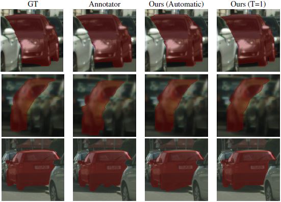
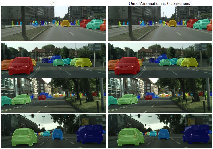
In addition, most of the comparisons with human annotators show that the method is at par with human-level annotation.
-
Figure 6: Qualitative results: comparison with human annotator.
-
Figure 7: Qualitative results: comparison with human annotator.
Conclusion
The important conclusions from this paper are:
1. The paper presented a powerful generic annotation tool for modelling complex annotations as a simple polygon that works on different unseen datasets.
2. Significant improvement in annotation time can be achieved with the Polygon-RNN method itself (speed-up factor of 4.74).
3. However, the flexibility of having inputs from a human annotator helps increase the IoU for a certain range of clicks.
4. The model architecture has a down-sampling factor of 16 and the final output resolution and accuracy is sensitive to object size.
5. Another downside of the model architecture is that training time is increased due to the training of the CNN for the first vertex.
Critique
1. With the human annotator in the loop, the model speeds up the process of annotation by over 7 times which is perhaps a big cost and time cutting improvement for companies.
2. Given that this model uses the VGG16 architecture compared to the 50 layer ResNet in SharpMask, this method is quite efficient.
3. This paper requires training of an entire CNN for the first vertex and is inefficient in that sense as it introduces additional parameters adding to the computation time and resource demand.
4. The baseline methods have an upper hand compared to this model when it comes to larger objects since the nature of the down-scaled structure adopted by this model.
5. In terms of future work, elimination of the additional CNN for the first vertex as well as an enhanced architecture to remain insensitive to the size of the object to be annotated should be implemented.
6. Compared to other models, the model was shown to not perform as well for larger objects (see table 3). This is likely due to the fact that vertex location determination is done in a highly compressed (28x28) representation compared to the input image(224x224). For larger objects, bounding boxes are larger. Each vertex represents many pixels. When up-converted back to the input image/bounding box size these may lead to errors especially when considering a very precise evaluation metric (intersection over union) is used. Potentially, the results can be improved by considering a higher resolution for the internal representation or one that scales with the size of the bounding.
7. While the model outperforms the baseline for certain categories of object, it is surprising that it underperforms in categories such as 'bus' and 'train'. With human annotators in the loop, one would expect the model to outperform in all categories.
8. One of the major contributions of this paper lies on the fact that this paper presents a method that does have an applicable value in the real world. In the paper, it does show that it can greatly reduce the human labeling efforts, and with human collaboration, this algorithm can help us tackle the image labeling problem much more efficiently. However, it does not provide the theoretical explanation that why would an RNN work better than a CNN in this case, a more in-depth analysis would make the paper better.
