XGBoost: Difference between revisions
No edit summary |
|||
| (21 intermediate revisions by 3 users not shown) | |||
| Line 6: | Line 6: | ||
== Introduction == | == Introduction == | ||
Brought to recognition by Tianqi Chen and Carlos Guestrin, eXtreme Gradient Boosting proves to be a highly scalable tree based supervised machine learning algorithm. Built up from the tree gradient boosting algorithm, it can be used to solve problems such as classification, regression and ranking problems in a more space and time efficient manner. This is achieved with the following modifications: <br> | |||
* The regularized objective function, which we aim to minimize, has two additional overfitting prevention techniques applied to it; shrinkage and column subsampling. | |||
* A novel distributed weighted quantile sketch is used to find candidate split points in weighted datasets and a default direction is introduced in each node to handle sparse data, which approximates the exact greedy algorithm for finding the best split. | |||
* Data is stored in blocks, which allows for parallel processing and for the quantile finding step to be reduced to linear time. The block size is also optimized to reduce cache misses when pre-fetching with a cache-aware prefetching algorithm for the exact greedy algorithm. | |||
== Related Works == | |||
XGBoost is built up from gradient boosting, which has been previously proven to be effective in solving classifcation, ranking and structured prediction problems.<br> | |||
It incorporates several techniques similar to or borrowed from previous works:<br> | |||
* Regularized model for overfitting prevention, similar to one used in regularized greedy forest. | |||
* Column sampling used in Random Forest. | |||
* Sparsity aware learning in linear models. | |||
* Tree learning parallelization; applying an exact greedy algorithm on column-partitioned data. | |||
* Finding quantile summary on (unweighted) data. | |||
== Tree Boosting In A Nutshell == | == Tree Boosting In A Nutshell == | ||
The author reviews gradient tree boosting in this section. | The author reviews gradient tree boosting in this section. | ||
| Line 20: | Line 33: | ||
The first term <math>l</math> is a differentiable convex loss function that calculates the measures between <math>\hat{y}</math> and <math>y</math>.<br> | The first term <math>l</math> is a differentiable convex loss function that calculates the measures between <math>\hat{y}</math> and <math>y</math>.<br> | ||
The second term <math>\Omega</math> penalizes on the complexity of model (the <math>f_k</math>'s). For a given tree (<math>f_k</math>), <math>T</math> is the number of leaves, and <math>\omega</math> is the leaf weights.<br> | The second term <math>\Omega</math> penalizes on the complexity of model (the <math>f_k</math>'s). For a given tree (<math>f_k</math>), <math>T</math> is the number of leaves, and <math>\omega</math> is the leaf weights.<br> | ||
The | The term <math>\gamma T</math> encourages the tree to be small, and the L2 regularization term <math>\frac{1}{2}\lambda ||\omega||^2</math> encourages the tree to have small weights.<br> | ||
=== Gradient Tree Boosting === | === Gradient Tree Boosting === | ||
| Line 62: | Line 75: | ||
The basic exact greedy algorithm is a split finding algorithm that is computationally expensive because it enumerates over all the possible splits for continuous features. It is impossible to be done efficiently when the memory is not enough to hold the data needed. A way to carry out this algorithm efficiently is to sort the data according to feature values and visit the data in order to accumulate the gradient statistics. The algorithm is shown below: | The basic exact greedy algorithm is a split finding algorithm that is computationally expensive because it enumerates over all the possible splits for continuous features. It is impossible to be done efficiently when the memory is not enough to hold the data needed. A way to carry out this algorithm efficiently is to sort the data according to feature values and visit the data in order to accumulate the gradient statistics. The algorithm is shown below: | ||
[[File: | [[File:algo1xg.png|frame|center|alt=Alt text|Basic Exact Greedy Algorithm]] | ||
=== Approximate Algorithm === | === Approximate Algorithm === | ||
| Line 68: | Line 81: | ||
The paper introduced a more efficient algorithm compared to Basic Exact Greedy Algorithm which is the Approximate Algorithm. The Approximate Algorithm first proposes candidate splitting points according to percentiles of feature distribution. It then maps the continuous features into buckets split by candidate points, aggregates the statistics and finds the best solution among proposals based on the aggregated statistics. The algorithm is shown below: | The paper introduced a more efficient algorithm compared to Basic Exact Greedy Algorithm which is the Approximate Algorithm. The Approximate Algorithm first proposes candidate splitting points according to percentiles of feature distribution. It then maps the continuous features into buckets split by candidate points, aggregates the statistics and finds the best solution among proposals based on the aggregated statistics. The algorithm is shown below: | ||
[[File: | [[File:algo2xg.png|frame|center|alt=Alt text|Approximate Algorithm]] | ||
There are also two variants to this algorithm, the global variant proposes all the candidate splits during the initial phase of tree construction and uses the same proposals for split finding at all levels. Whereas, the local variant re-proposes after each split. The global variant usually requires less proposal steps but uses more candidate points than local variant because candidates are not refined after each split. For deeper trees, usage of local variant may be more appropriate as compared to global variant. The figure below shows the a comparison in accuracy between Basic Exact Greedy and Approximate split finding algorithms with different variant over the number of iterations. We can see that the quantile strategy is able to achieve similar accuracy as the Basic Exact Greedy algorithm given a reasonable approximation level. | There are also two variants to this algorithm, the global variant proposes all the candidate splits during the initial phase of tree construction and uses the same proposals for split finding at all levels. Whereas, the local variant re-proposes after each split. The global variant usually requires less proposal steps but uses more candidate points than local variant because candidates are not refined after each split. For deeper trees, usage of local variant may be more appropriate as compared to global variant. The figure below shows the a comparison in accuracy between Basic Exact Greedy and Approximate split finding algorithms with different variant over the number of iterations. We can see that the quantile strategy is able to achieve similar accuracy as the Basic Exact Greedy algorithm given a reasonable approximation level. | ||
[[File: | [[File:accuracyxg.png|frame|center|alt=Alt text|Comparison of accuracy between different algorithms]] | ||
=== Weighted Quantile Sketch === | === Weighted Quantile Sketch === | ||
| Line 104: | Line 117: | ||
In order to solve the sparsity present in the dataset, we suggest to add a default direction in each tree node will classified into when there is a missing value in the matrix of the dataset. This is demonstrated in the figure below: | In order to solve the sparsity present in the dataset, we suggest to add a default direction in each tree node will classified into when there is a missing value in the matrix of the dataset. This is demonstrated in the figure below: | ||
[[File:defaultdirection.png|frame|center|alt=Alt text|Default Direction for missing value]] | |||
The algorithm below helps us to calculate the optimal direction to proceed in each branch. Beside that, it also allows user to set a range for the accepted value and neglect the out-of-range value when calculating the score. | |||
[[File:algo3xg.png|frame|center|alt=Alt text|Sparsity-aware Split Finding Algorithm]] | |||
The figure below shows the difference in time needed per tree over number of threads between Sparsity Aware algorithm compared to a basic algorithm on a sparse dataset Allstate-10K, the sparsity was caused by feature engineering using one-hot encoding. | |||
[[File: | [[File:fig5xg.png|frame|center|alt=Alt text|Sparsity-aware Algorithm vs Basic Algorithm on sparse data]] | ||
== System Design == | == System Design == | ||
| Line 209: | Line 229: | ||
== Conclusion == | == Conclusion == | ||
This paper thoroughly examines how XGBoost, a tree based supervised machine learning algorithm, proves to be highly scalable. To the existing tree boosting system, it introduces the addition of algorithmic optimizations, such as a sparsity-aware algorithm and weighted quantile sketch for split finding, and important system design implementations, such as an optimal block structure with cache-awareness for out-of-core tree learning. XGBoost is experimented on with four datasets, which evaluates its outstanding performance in comparison to several other exact greedy tree boosting implementations. Hence, XGBoost is suitable to solve real-world scale problems with minimal resources. | |||
== References == | == References == | ||
Latest revision as of 02:21, 5 December 2021
Presented by
- Chun Waan Loke
- Peter Chong
- Clarice Osmond
- Zhilong Li
Introduction
Brought to recognition by Tianqi Chen and Carlos Guestrin, eXtreme Gradient Boosting proves to be a highly scalable tree based supervised machine learning algorithm. Built up from the tree gradient boosting algorithm, it can be used to solve problems such as classification, regression and ranking problems in a more space and time efficient manner. This is achieved with the following modifications:
- The regularized objective function, which we aim to minimize, has two additional overfitting prevention techniques applied to it; shrinkage and column subsampling.
- A novel distributed weighted quantile sketch is used to find candidate split points in weighted datasets and a default direction is introduced in each node to handle sparse data, which approximates the exact greedy algorithm for finding the best split.
- Data is stored in blocks, which allows for parallel processing and for the quantile finding step to be reduced to linear time. The block size is also optimized to reduce cache misses when pre-fetching with a cache-aware prefetching algorithm for the exact greedy algorithm.
Related Works
XGBoost is built up from gradient boosting, which has been previously proven to be effective in solving classifcation, ranking and structured prediction problems.
It incorporates several techniques similar to or borrowed from previous works:
- Regularized model for overfitting prevention, similar to one used in regularized greedy forest.
- Column sampling used in Random Forest.
- Sparsity aware learning in linear models.
- Tree learning parallelization; applying an exact greedy algorithm on column-partitioned data.
- Finding quantile summary on (unweighted) data.
Tree Boosting In A Nutshell
The author reviews gradient tree boosting in this section.
Regularized Learning Objective
The author first gives the prediction equation (1) and the regularized objective (2).
(1) The additive prediction model is given as
[math]\displaystyle{ \hat{y_i}=\sum_{k=1}^{K}f_k(x_i), f_k \in \mathcal{F} }[/math]
where each [math]\displaystyle{ f_k }[/math] corresponds to an independent tree structure with its weights, and [math]\displaystyle{ \mathcal{F} }[/math] is the "space of regression trees"
(2) The regularized objective to be minimized is given as
[math]\displaystyle{ \mathcal{L}=\sum_{i}l(\hat{y_i},y_i)+\sum_k \Omega(f_k) }[/math] where [math]\displaystyle{ \Omega(f)=\gamma T+\frac{1}{2}\lambda ||\omega||^2 }[/math]
The first term [math]\displaystyle{ l }[/math] is a differentiable convex loss function that calculates the measures between [math]\displaystyle{ \hat{y} }[/math] and [math]\displaystyle{ y }[/math].
The second term [math]\displaystyle{ \Omega }[/math] penalizes on the complexity of model (the [math]\displaystyle{ f_k }[/math]'s). For a given tree ([math]\displaystyle{ f_k }[/math]), [math]\displaystyle{ T }[/math] is the number of leaves, and [math]\displaystyle{ \omega }[/math] is the leaf weights.
The term [math]\displaystyle{ \gamma T }[/math] encourages the tree to be small, and the L2 regularization term [math]\displaystyle{ \frac{1}{2}\lambda ||\omega||^2 }[/math] encourages the tree to have small weights.
Gradient Tree Boosting
Let [math]\displaystyle{ \hat{y_i}^{(t)} }[/math] be the prediction of [math]\displaystyle{ y_i }[/math] at the t-th iteration.
Since the prediction equation is simply additive, [math]\displaystyle{ {\hat y_i}^{(t)}=\hat{y_{i}}^{(t-1)}+f_t(x_i) }[/math]
Using this equation and 2nd order Taylor approximation on the loss function [math]\displaystyle{ l(y_i,\hat{y_i}^{(t-1)}) }[/math] gives
\begin{align}
\mathcal{L}^{(t)}&=\sum_{i}^{n}l(y_i,\hat{y_i}^{(t-1)}+f_t(x_i))+\Omega(f_t)\\
&\simeq \sum_{i}^{n}[l(y_i,\hat{y_i}^{(t-1)})+g_if_t(x_i)+\frac{1}{2}h_if_t^2(x_i)]+\gamma T+\frac{1}{2}\lambda \sum_{j=1}^{T}\omega^2\\
\end{align}
where [math]\displaystyle{ g_i }[/math] and [math]\displaystyle{ h_i }[/math] are the first and second derivative of the loss function [math]\displaystyle{ l(y_i,\hat{y_i}^{(t-1)}) }[/math] with repspect to the term [math]\displaystyle{ \hat{y}^{(t-1)} }[/math]
We can simplify this objective by removing the constant term [math]\displaystyle{ l(y_i,\hat{y_i}^{(t-1)}) }[/math].
Define [math]\displaystyle{ I_j=\{i|q(x_i)=j\} }[/math], where [math]\displaystyle{ q }[/math] is the tree structure. Since every [math]\displaystyle{ x_i }[/math] is mapped by [math]\displaystyle{ q }[/math] to some leaf [math]\displaystyle{ j }[/math], going through every [math]\displaystyle{ x_i }[/math] is equivalent to going through each leaf j of the structure.
\begin{align}
\tilde{\mathcal{L}}^{(t)}&= \sum_{i}^{n}[g_if_t(x_i)+\frac{1}{2}h_if_t^2(x_i)]+\gamma T+\frac{1}{2}\lambda \sum_{j=1}^{T}\omega^2\\
&= \sum_{j=1}^{T}[(\sum_{i \in I_j}g_i)\omega_j+\frac{1}{2}(\sum_{i \in I_j}h_i+\lambda)\omega_j^2]+\gamma T
\end{align}
Then for a fixed structure [math]\displaystyle{ q }[/math], the optimal weight of leaf [math]\displaystyle{ j }[/math] and the optimal objective value are given as
\begin{align}
\omega_j^{*} &= -\frac{\sum_{i \in I_j}g_i}{\sum_{i \in I_j}h_i+\lambda}\\
\tilde{\mathcal{L}}^{(t)}(q) &=-\frac{1}{2}\sum_{j=1}^{T}\frac{(\sum_{i \in I_j}g_i)^2}{\sum_{i \in I_j}h_i+\lambda}+\gamma T
\end{align}
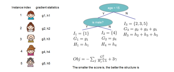
Instead of enumerating through all possible tree structures q, a greedy algorithm of iteratively adding branches is used.
Let [math]\displaystyle{ I_L }[/math] and [math]\displaystyle{ I_R }[/math] be the instance sets of left and right nodes after split and let [math]\displaystyle{ I=I_L\cup I_R }[/math].
The loss reduction after split is given by
\begin{align}
\tilde{\mathcal{L}}_{\text{split}} &=\frac{1}{2}[\frac{(\sum_{i \in I_L}g_i)^2}{\sum_{i \in I_L}h_i+\lambda}+\frac{(\sum_{i \in I_R}g_i)^2}{\sum_{i \in I_R}h_i+\lambda}-\frac{(\sum_{i \in I}g_i)^2}{\sum_{i \in I}h_i+\lambda}]+\gamma
\end{align}
Shrinkage and Column Subsampling
The author also mentioned two other methods in order to avoid over-fitting.
(1) Shrinkage. Similar to the learning rate in stochastic optimization, a new weight is added to each tree boosting to reduce the influence of a single tree and leave space for future trees.
(2) Column (feature) subsampling. In the paper, the author only mentioned that this technique speeds up parallel algorithm used in later sections.
Split Finding Algorithms
It is very important to find the best split for tree learning to perform well. Here are a few split finding algorithms mentioned in the paper:
Basic Exact Greedy Algorithm
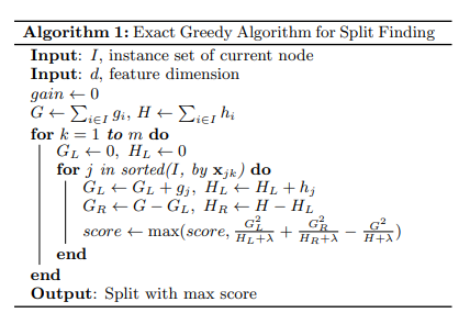
The basic exact greedy algorithm is a split finding algorithm that is computationally expensive because it enumerates over all the possible splits for continuous features. It is impossible to be done efficiently when the memory is not enough to hold the data needed. A way to carry out this algorithm efficiently is to sort the data according to feature values and visit the data in order to accumulate the gradient statistics. The algorithm is shown below:
Approximate Algorithm
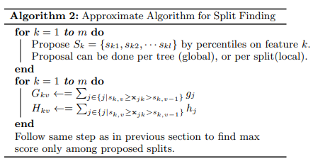
The paper introduced a more efficient algorithm compared to Basic Exact Greedy Algorithm which is the Approximate Algorithm. The Approximate Algorithm first proposes candidate splitting points according to percentiles of feature distribution. It then maps the continuous features into buckets split by candidate points, aggregates the statistics and finds the best solution among proposals based on the aggregated statistics. The algorithm is shown below:
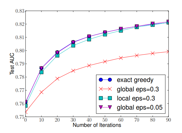
There are also two variants to this algorithm, the global variant proposes all the candidate splits during the initial phase of tree construction and uses the same proposals for split finding at all levels. Whereas, the local variant re-proposes after each split. The global variant usually requires less proposal steps but uses more candidate points than local variant because candidates are not refined after each split. For deeper trees, usage of local variant may be more appropriate as compared to global variant. The figure below shows the a comparison in accuracy between Basic Exact Greedy and Approximate split finding algorithms with different variant over the number of iterations. We can see that the quantile strategy is able to achieve similar accuracy as the Basic Exact Greedy algorithm given a reasonable approximation level.
Weighted Quantile Sketch
Proposing candidate split points is the most important step in the Approximate Algorithm, it is done by using the percentile of a feature to make candidates distribute evenly on a dataset.
Formally, we have a dataset
[math]\displaystyle{ D_k={(x_{1k},h_1),(x_{2k},h_2),...,(x_{nk},h_n)} }[/math]
where [math]\displaystyle{ x_i }[/math]'s are the feature values of each data point and [math]\displaystyle{ h_i }[/math]'s represents the weight of the corresponding feature [math]\displaystyle{ x_i }[/math].
Then, we can use the following rank function to compute [math]\displaystyle{ r_k(z) }[/math], the proportion of instances whose feature value among [math]\displaystyle{ (x_i,...,x_k) }[/math] is smaller than data point [math]\displaystyle{ z }[/math].
[math]\displaystyle{ r_k(z) = \frac{1}{\sum_{(x,h) \in D_k} h} \displaystyle\sum_{(x,h) \in D_k, x\lt z} h, }[/math]
The objective here is to find candidate split points [math]\displaystyle{ {s_{k1}, s_{k2}, …, s_{kl}} }[/math], such that:
[math]\displaystyle{ |r_k(s_{k,j}) – r_k(s_{k,j+1})| \lt \epsilon, s_{k1} = \displaystyle\min_i x_{ik}, s_{kl} = \displaystyle\max_{i} x_{ik}, \forall i }[/math]
Where [math]\displaystyle{ \epsilon }[/math] is an approximation factor. Usually, it should approximately have [math]\displaystyle{ \frac{1}{\epsilon} }[/math] splitting points.
Sparsity-aware Split Finding
Typically in real world situation, it is quite common that our dataset is sparse. Some of the possible causes are:
- Missing values in the data
- Huge amount of zero entries present in the data
- Artifacts of feature engineering (e.g. One-hot encoding)
In order to solve the sparsity present in the dataset, we suggest to add a default direction in each tree node will classified into when there is a missing value in the matrix of the dataset. This is demonstrated in the figure below:

The algorithm below helps us to calculate the optimal direction to proceed in each branch. Beside that, it also allows user to set a range for the accepted value and neglect the out-of-range value when calculating the score.
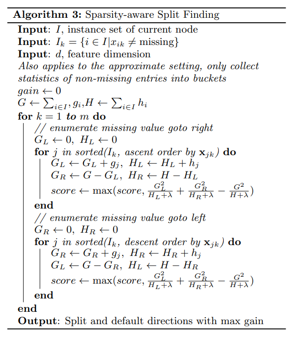
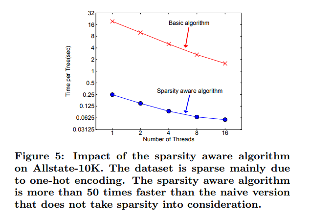
The figure below shows the difference in time needed per tree over number of threads between Sparsity Aware algorithm compared to a basic algorithm on a sparse dataset Allstate-10K, the sparsity was caused by feature engineering using one-hot encoding.
System Design
Column Block for Parallel Learning
The most time consuming part of tree learning is to get the data into sorted order. To overcome this problem, XGBoost stores the data in blocks where each block performs the sorting operation in parallel. The results are then merged together.
- For the exact greedy algorithm, XGBoost stores the entire dataset in a single block
- Original spase aware algorithm costs: [math]\displaystyle{ O(Kd∥x∥_0 log(n)) }[/math]
- Tree boosting on block structure costs: [math]\displaystyle{ O(Kd∥x∥_0 + ∥x∥_0 log(n)) }[/math]
- Hence, block structure helps to save an additional [math]\displaystyle{ log(n) }[/math] factor
- For approximate algorithms, XGBoost stores the dataset in multiple blocks
- Original algorithm with binary search costs: [math]\displaystyle{ O(Kd∥x∥_0 log(q)) }[/math]
- With block structure costs: [math]\displaystyle{ O(Kd∥x∥_0 + ∥x∥_0 log(B)) }[/math]
- Hence, block structure helps to save an additional [math]\displaystyle{ log(q) }[/math] factor
K = total number of trees
d = maximum depth of the tree
[math]\displaystyle{ ∥x∥_0 }[/math] = number of non-missing entries in the training data
n = number of rows in the dataset
q = number of proposal candidates in the dataset, usually between 32 to 100
B = maximum number of rows in each block

Cache-aware Access
The proposed block structure optimizes the computation complexity but requires indirect fetches of gradient statistics by row index. XGBoost optimizes the process by using the following methods.
- For the exact greedy algorithm, XGBoost uses a cache-aware prefetching algorithm
- It stores Gradient and Hessians in the cache to make calculations fast
- It runs twice as fast as the naive method when the dataset is large
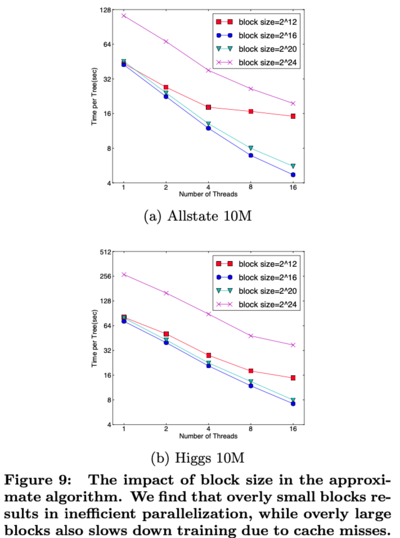
- For approximate algorithms, XGBoost chooses a specific block size
- Choosing a small block size results in inefficient parallelization
- Choosing a large block size results in cache misses
- Various choices of block size are compared and the results are shown in Figure 9
- XGBoost chose [math]\displaystyle{ 2^{16} }[/math] as the block size
Blocks for Out-of-core Computation
When the dataset is too large for the cache and main memory, XGBoost utilizes disk spaces as well. Since reading and writing data to the disks are slow, XGBoost optimizes the process by using the following two methods.
- Block Compression
- Blocks are compressed by columns
- Although decompressing takes time, it is still faster than reading from the disks
- Block Sharding
- If multiple disks are available, data is split into those disks
- When the CPU needs data, all the disks can be read at the same time
End To End Evaluations
System Implementation
XGBoost is a portable and reusable open-source package. It supports:
- various weighted classification
- various objective functions (rank & user defined)
- popular languages (python, R, Julia)
- data science pipelines (scikit-learn)
- big data stacks (Flink, Spark)
- cloud platform (Tianchi8)
Dataset and Setup
A summary of the 4 datasets used in the experiments is in table 2.

The first and last datasets were used specifically to evaluate the impact of sparsity-aware algorithm and the scaling property of the system in the out-of-core and the distributed settings respectively. In all of the experiments, common settings such as maximum depth equal to 8, shrinkage equal to 0.1 and no column subsampling are applied.
Classification
A subset (n = 1M) of Higgs Boson dataset was used for classification. The results are shown in Table 3.

- R’s GBM creates a tree fast by using greedy approach that only expands one branch of a tree but with the cost of lower accuracy
- XGBoost and scikit-learn have better performance than R’s GBM
- XGBoost runs more than 10x faster than scikit-learn in learning a full tree
- Column subsamples give slightly worse performance possibly due to a few important features in this dataset.
Learning to Rank
The results in comparing XGBoost with pGBRT are shown in Table 4.

- XGBoost runs exact greedy algorithm while pGBRT only supports an approximate algorithm
- XGBoost runs faster
- Subsampling column reduces running time and gives higher performance possibly due to preventing overfitting
Out-of-core Experiment
An extremely large Criteo dataset was used to evaluate the out-of-core setting. The results are shown in the figure below.
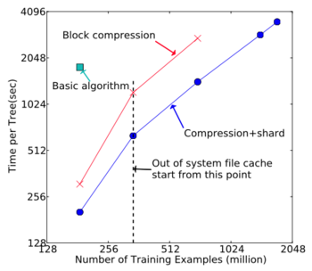
- Compression speed up the computation by a factor of 3
- Sharding into 2 disks further gives 2x speed
Distributed Experiment
YARN cluster on EC2 with m3.2xlarge machines was used to evaluate the distributed setting. XGBoost was compared with Spark MLLib and H20.
- XGBoost can switch to out-of-core setting when the memory runs out, while the baseline systems need to store the data in RAM
- XGBoost runs faster than the baseline systems
- The baseline systems are only able to handle a subset of the data with the given resources while XGBoost was able to scale smoothly to all 1.7B rows
- XGBoost’s performance scales linearly with more machines
- XGBoost is able to handle all 1.7B data with only 4 machines
Conclusion
This paper thoroughly examines how XGBoost, a tree based supervised machine learning algorithm, proves to be highly scalable. To the existing tree boosting system, it introduces the addition of algorithmic optimizations, such as a sparsity-aware algorithm and weighted quantile sketch for split finding, and important system design implementations, such as an optimal block structure with cache-awareness for out-of-core tree learning. XGBoost is experimented on with four datasets, which evaluates its outstanding performance in comparison to several other exact greedy tree boosting implementations. Hence, XGBoost is suitable to solve real-world scale problems with minimal resources.
References
[1] R. Bekkerman. The present and the future of the kdd cup competition: an outsider’s perspective.
[2] R. Bekkerman, M. Bilenko, and J. Langford. Scaling Up Machine Learning: Parallel and Distributed Approaches. Cambridge University Press, New York, NY, USA, 2011.
[3] J. Bennett and S. Lanning. The netflix prize. In Proceedings of the KDD Cup Workshop 2007, pages 3–6, New York, Aug. 2007.
[4] L. Breiman. Random forests. Maching Learning, 45(1):5–32, Oct. 2001.
[5] C. Burges. From ranknet to lambdarank to lambdamart: An overview. Learning, 11:23–581, 2010.
[6] O. Chapelle and Y. Chang. Yahoo! Learning to Rank Challenge Overview. Journal of Machine Learning Research - W & CP, 14:1–24, 2011.
[7] T. Chen, H. Li, Q. Yang, and Y. Yu. General functional matrix factorization using gradient boosting. In Proceeding of 30th International Conference on Machine Learning (ICML’13), volume 1, pages 436–444, 2013.
[8] T. Chen, S. Singh, B. Taskar, and C. Guestrin. Efficient second-order gradient boosting for conditional random fields. In Proceeding of 18th Artificial Intelligence and Statistics Conference (AISTATS’15), volume 1, 2015.
[9] R.-E. Fan, K.-W. Chang, C.-J. Hsieh, X.-R. Wang, and C.-J. Lin. LIBLINEAR: A library for large linear classification. Journal of Machine Learning Research, 9:1871–1874, 2008.
[10] J. Friedman. Greedy function approximation: a gradient boosting machine. Annals of Statistics, 29(5):1189–1232, 2001.
[11] J. Friedman. Stochastic gradient boosting. Computational Statistics & Data Analysis, 38(4):367–378, 2002.
[12] J. Friedman, T. Hastie, and R. Tibshirani. Additive logistic regression: a statistical view of boosting. Annals of Statistics, 28(2):337–407, 2000.
[13] J. H. Friedman and B. E. Popescu. Importance sampled learning ensembles, 2003.
[14] M. Greenwald and S. Khanna. Space-efficient online computation of quantile summaries. In Proceedings of the 2001 ACM SIGMOD International Conference on Management of Data, pages 58–66, 2001.
[15] X. He, J. Pan, O. Jin, T. Xu, B. Liu, T. Xu, Y. Shi, A. Atallah, R. Herbrich, S. Bowers, and J. Q. n. Candela. Practical lessons from predicting clicks on ads at facebook. In Proceedings of the Eighth International Workshop on Data Mining for Online Advertising, ADKDD’14, 2014.
[16] P. Li. Robust Logitboost and adaptive base class (ABC) Logitboost. In Proceedings of the Twenty-Sixth Conference Annual Conference on Uncertainty in Artificial Intelligence (UAI’10), pages 302–311, 2010.
[17] P. Li, Q. Wu, and C. J. Burges. Mcrank: Learning to rank using multiple classification and gradient boosting. In Advances in Neural Information Processing Systems 20, pages 897–904. 2008.
[18] X. Meng, J. Bradley, B. Yavuz, E. Sparks, S. Venkataraman, D. Liu, J. Freeman, D. Tsai, M. Amde, S. Owen, D. Xin, R. Xin, M. J. Franklin, R. Zadeh, M. Zaharia, and A. Talwalkar. MLlib: Machine learning in apache spark. Journal of Machine Learning Research, 17(34):1–7, 2016.
[19] B. Panda, J. S. Herbach, S. Basu, and R. J. Bayardo. Planet: Massively parallel learning of tree ensembles with mapreduce. Proceeding of VLDB Endowment, 2(2):1426–1437, Aug. 2009.
[20] F. Pedregosa, G. Varoquaux, A. Gramfort, V. Michel, B. Thirion, O. Grisel, M. Blondel, P. Prettenhofer, R. Weiss, V. Dubourg, J. Vanderplas, A. Passos, D. Cournapeau, M. Brucher, M. Perrot, and E. Duchesnay. Scikit-learn: Machine learning in Python. Journal of Machine Learning Research, 12:2825–2830, 2011.
[21] G. Ridgeway. Generalized Boosted Models: A guide to the gbm package.
[22] S. Tyree, K. Weinberger, K. Agrawal, and J. Paykin. Parallel boosted regression trees for web search ranking. In Proceedings of the 20th international conference on World wide web, pages 387–396. ACM, 2011.
[23] J. Ye, J.-H. Chow, J. Chen, and Z. Zheng. Stochastic gradient boosted distributed decision trees. In Proceedings of the 18th ACM Conference on Information and Knowledge Management, CIKM ’09.
[24] Q. Zhang and W. Wang. A fast algorithm for approximate quantiles in high speed data streams. In Proceedings of the 19th International Conference on Scientific and Statistical Database Management, 2007.
[25] T. Zhang and R. Johnson. Learning nonlinear functions using regularized greedy forest. IEEE Transactions on Pattern Analysis and Machine Intelligence, 36(5), 2014.