Self-Supervised Learning of Pretext-Invariant Representations: Difference between revisions
No edit summary |
|||
| (42 intermediate revisions by 13 users not shown) | |||
| Line 1: | Line 1: | ||
==Authors== | |||
Ishan Misra, Laurens van der Maaten | |||
== Presented by == | == Presented by == | ||
| Line 5: | Line 8: | ||
== Introduction == | == Introduction == | ||
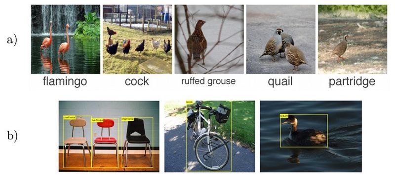
Modern image recognition and object detection systems find image representations using a large number data with pre-defined semantic | Modern image recognition and object detection systems find image representations by using a large number of data points with pre-defined semantic annotations. Examples of these annotations include class labels [1] and bounding boxes [2], as shown in Figure 1. There is a need for a large amount of labeled data, which is often very difficult to obtain. Also, these systems usually learn specific features for a particular type of class and not necessarily semantically meaningful features that can help generalize to other domains and classes. In other words, '''pre-defined semantic annotations scale poorly to the long tail of visual concepts'''[3]. Therefore, there has been a big interest in the community for learning image representations that are more visually meaningful and can help in a variety of tasks, such as image recognition and object detection. One of the fast-growing areas of research that tries to address this problem is '''self-supervised Learning'''. Self-Supervised Learning tries to learn meaningful semantics by just using the inputs themselves rather than using pre-defined semantic annotated data. As will show, the self-supervised learning paradigm removes the need for using human-provided class labels or bounding boxes for classification and object detection tasks, respectively. | ||
[[File: SSL_1.JPG | 800px | center]] | [[File: SSL_1.JPG | 800px | center]] | ||
<div align="center">'''Figure 1:''' Semantic Annotations used for finding image representations: a) Class labels and b) Bounding Boxes </div> | <div align="center">'''Figure 1:''' Semantic Annotations used for finding image representations: a) Class labels and b) Bounding Boxes </div> | ||
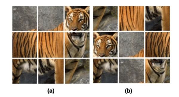
Self-Supervised Learning is often done using a set of tasks called ''' | Self-Supervised Learning is often done using a set of tasks called '''pretext tasks'''. During these tasks, a transformation <math> \tau </math> is applied to unlabeled images <math> I </math> to obtain a set of transformed images, <math> I^{t} </math>. Then, a deep neural network, <math> \phi(\theta) </math>, is trained to predict some characteristic of the transformation from the transformed image. Several pretext tasks exist based on the type of transformation used. For example, if a neural network can accurately determine if an image is upside down or not, then perhaps it has learned some semantically meaningful representation of the image. This pre-empts the need for human-provided labels. Two of the most common pretext tasks used are rotations and jigsaw puzzle [4,5,6]. As shown in Figure 2, in the rotation task, unlabeled images, <math> </math> are rotated by random degrees (0,90,180,270) and the deep network learns to predict the rotation degree. The jigsaw task is more complicated than the rotation prediction task; first unlabeled images are cropped into 9 patches, then the image is perturbed by randomly permuting the nine patches. The unlabeled original image is referred to as the anchor data point (Figure 3-a), the reshuffled image that we get by permuting patches will be our positive sample (Figure 3-b) and the rest of the images in the dataset will be considered as negative samples. Each permutation falls into one of the 35 classes according to a formula given by the authors. A deep network is then trained to predict the class of the permutation of the patches in the perturbed image. Some other tasks include colorization, where the model tries to revert the colors of a colored image turned to grayscale, and image reconstruction where a square chunk of the image is deleted and the model tries to reconstruct that part. | ||
[[File: SSL_2.JPG |1000px | center]] | [[File: SSL_2.JPG |1000px | center]] | ||
<div align="center">'''Figure 2:''' Self-Supervised Learning using Rotation and Jigsaw Pretext Tasks </div> | <div align="center">'''Figure 2:''' Self-Supervised Learning using Rotation and Jigsaw Pretext Tasks </div> | ||
Although the proposed pretext tasks have | [[File:figure3.jpg |600px | center]] | ||
<div align="center">'''Figure 3:''' Jigsaw puzzle used as a pretext task in unsupervised representation learning. (a) Original image (b) augmented image </div> | |||
Although the proposed pretext tasks have achieved promising results, they have the disadvantage of being covariant to the applied transformation. In other words, as deep networks are trained to predict transformation characteristics, they will also learn representations that will vary based on the applied transformation. By intuition, we would like to obtain representations that are common between the original images and the transformed ones. This idea is supported by the fact that humans can recognize these transformed images. For example, a human can identify a permuted image of a tiger (as in figure 3) as a "permuted tiger" as well as the original image as a "tiger". Thus, the "tiger" aspect of the representations human learn is invariant to the transform, which cannot be taken for granted in standard self-supervision. The paper tries to address this problem by introducing '''Pretext Invariant Representation Learning''' (PIRL) that obtains representations which are transformation invariant and therefore more semantically meaningful. The performance of the proposed method is evaluated on several self-supervision learning benchmarks. The results show that the PIRL introduces a new state-of-the-art method in self-supervised Learning by learning transformation invariant representations. | |||
== Problem Formulation and Methodology == | == Problem Formulation and Methodology == | ||
[[File: SSL_3.JPG | 800px | center]] | [[File: SSL_3.JPG | 800px | center]] | ||
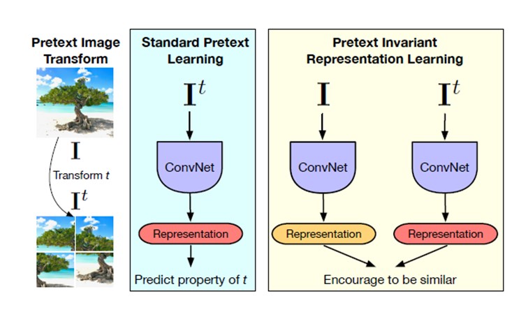
<div align="center">'''Figure 3:''' | <div align="center">'''Figure 3:''' Overview of Standard Pretext Learning and Pretext-Invariant Representation Learning (PIRL). </div> | ||
An overview of the proposed method and a comparison with Pretext Tasks are shown in Figure 3. For a given image ,<math>I</math>, in the | An overview of the proposed method and a comparison with Pretext Tasks are shown in Figure 3. For a given image , <math>I</math>, in the dataset of unlabeled images, <math> D=\{{I_1,I_2,...,I_{|D|}}\} </math>, a transformation <math> \tau </math> is applied: | ||
\begin{align} \tag{1} \label{eqn:1} | \begin{align} \tag{1} \label{eqn:1} | ||
| Line 32: | Line 37: | ||
\begin{align} \tag{2} \label{eqn:2} | \begin{align} \tag{2} \label{eqn:2} | ||
l_{\text{cov}}(\theta,D)=\frac{1}{|D|} \sum_{I \in {D}}^{} L(v_I,z(t) | l_{\text{cov}}(\theta,D)=\frac{1}{|D|} \sum_{I \in {D}}^{} L(v_I,z(t)) | ||
\end{align} | \end{align} | ||
As it can be seen, the loss function covaries with the applied transformation and therefore, the obtained representations may not be semantically meaningful. PIRL tries to solve for this problem as shown in Figure 3. The original and transformed images are passed through two parallel convolutional neural networks to obtain two | As it can be seen, the loss function covaries with the applied transformation and therefore, the obtained representations may not be semantically meaningful. PIRL tries to solve for this problem as shown in Figure 3. The original and transformed images are passed through two parallel convolutional neural networks to obtain two sets of representations, <math>v(I)</math> and <math>v(I^t)</math>. Then, a contrastive loss function is defined to ensure that the representations of the original and transformed images are similar to each other. The transformation invariant loss function can be defined as: | ||
\begin{align} \tag{3} \label{eqn:3} | \begin{align} \tag{3} \label{eqn:3} | ||
| Line 44: | Line 49: | ||
\begin{align} \tag{4} \label{eqn:4} | \begin{align} \tag{4} \label{eqn:4} | ||
h(v_I,v_{I^t})=\frac{\exp \biggl( \frac{s(v_I,v_{I^t}}{\tau} | h(v_I,v_{I^t})=\frac{\exp \biggl( \frac{s(v_I,v_{I^t})}{\tau} \biggr)}{\exp \biggl(\frac{s(v_I,v_{I^t})}{\tau} \biggr) + \sum_{I^{'} \in D_N}^{} \exp \biggl( \frac{s(v_{I^t},v_{I^{'}})}{\tau} \biggr)} | ||
\end{align} | \end{align} | ||
where <math>s(.,.)</math> is the cosine similarity function and <math>\tau</math> is the temperature parameter that is usually set to 0.07. Also, a set of N images are chosen randomly from dataset where <math>I^{'}\neq I</math>. These images are used in the loss in order to ensure their representation dissimilarity with transformed image representations. Also, during model implementation, two heads (few additional deep layers) , <math>f</math> and <math>g</math>, are applied on top of <math>v(I)</math> and <math>v(I^t)</math>. Using the NCE formulation, the contrastive loss can be written as: | where <math>s(.,.)</math> is the cosine similarity function and <math>\tau</math> is the temperature parameter that is usually set to 0.07. Also, a set of N images are chosen randomly from the dataset where <math>I^{'}\neq I</math>. These images are used in the loss in order to ensure their representation dissimilarity with transformed image representations. Also, during model implementation, two heads (few additional deep layers), <math>f</math> and <math>g</math>, are applied on top of <math>v(I)</math> and <math>v(I^t)</math>. Using the NCE formulation, the contrastive loss can be written as: | ||
\begin{align} \tag{5} \label{eqn:5} | \begin{align} \tag{5} \label{eqn:5} | ||
| Line 56: | Line 61: | ||
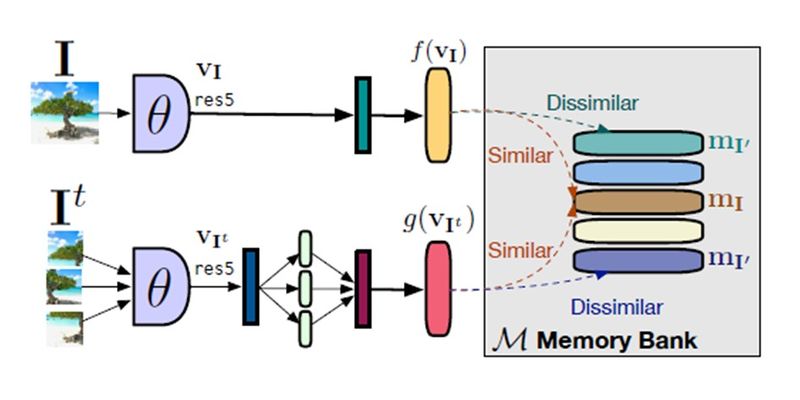
<div align="center">'''Figure 4:''' Proposed PIRL </div> | <div align="center">'''Figure 4:''' Proposed PIRL </div> | ||
Although the formulation looks complicated, the take | Although the formulation looks complicated, the take-away here is that by minimizing the NCE based loss function, the similarity between the original and transformed image representations, <math>v(I)</math> and <math>v(I^t)</math>, increases and at the same time the dissimilarity between <math>v(I^t)</math> and negative images representations, <math>v(I^{'})</math>, is increased. According to the previous work, an infeasibly large batch size is needed to obtain a large number of negatives. To tackle this problem, a memory bank [9], <math>M</math>, is used during training which contains feature representation <math>m_I</math> for each image in the dataset including the negative images. The proposed PIRL model is shown in Figure 4. Finally, the contrastive loss in equation \eqref{eqn:5} does not take into account the dissimilarity between the original image representations, <math>v(I)</math>, and the negative image representations, <math>v(I^{'})</math>. By taking this into account and using the memory bank, the final contrastive loss function is obtained as: | ||
\begin{align} \tag{6} \label{eqn:6} | \begin{align} \tag{6} \label{eqn:6} | ||
L(I,I^{t})=\lambda L_{\text{NCE}}(m_I,g(v_{I^t})) + (1-\lambda)L_{\text{NCE}}(m_I,f(v_{I})) | L(I,I^{t})=\lambda L_{\text{NCE}}(m_I,g(v_{I^t})) + (1-\lambda)L_{\text{NCE}}(m_I,f(v_{I})) | ||
\end{align} | \end{align} | ||
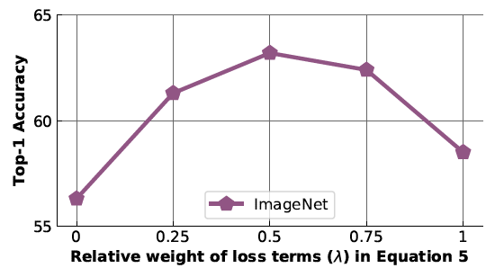
where <math>\lambda</math> is a hyperparameter that determines the weight of each of NCE losses. The default value for this parameter is 0.5. In the next section, experimental results are shown using the proposed PIRL model. | |||
==Experimental Results == | ==Experimental Results == | ||
For the experiments in this section, PIRL is implemented using jigsaw transformations. The combination of PIRL with other types of transformations is shown in the last section of the summary. The quality of image representations obtained from PIRL Self-Supervised Learning is evaluated by comparing its performance to other Self-Supervised Learning methods on image recognition and object detection tasks. For the experiments, a ResNet50 model is trained using PIRL and other methods by using 1.28M randomly sampled images from the ImageNet dataset. Also, the number of negative images used for PIRL is N=32000. | |||
===Object Detection=== | ===Object Detection=== | ||
A Faster R-CNN model with a ResNet-50 backbone, pre-trained using PIRL and other Self-Supervised methods, is employed for the object detection task. Then, the pre-trained model weights are used as initial weights for the Faster-RCNN model backbone during training on the VOC07+12 dataset. The result of object detection using PIRL is shown in Figure (5) and it is compared to other methods. It can be seen that PIRL not only outperforms other Self-Supervised-based methods, '''for the first time it outperforms Supervised Pre-training on object detection'''. They emphasize that PIRL achieves this result using the same backbone model, the same number of finetuning epochs, and the exact same pre-training data (but without the labels). This result is a substantial improvement over prior self-supervised approaches that obtain worse performance than fully supervised baselines despite using orders of magnitude more curated training data or much larger backbone models. | |||
[[File: SSL_5.PNG | 800px | center]] | [[File: SSL_5.PNG | 800px | center]] | ||
| Line 76: | Line 81: | ||
===Image Classification with linear models=== | ===Image Classification with linear models=== | ||
In the next experiment, the performance of the PIRL is evaluated on image classification using four different datasets. For this experiment, the ResNet-50 | In the next experiment, the performance of the PIRL is evaluated on image classification using four different datasets. For this experiment, the pre-trained ResNet-50 model is utilized as an image feature extractor. Then, a linear classifier is trained on fixed image representations. The results are shown in Figure (6). The results demonstrate that while PIRL substantially outperforms other Self-Supervised Learning methods, it still falls behind Supervised Pre-trained Learning. | ||
[[File: SSL_6.PNG | 800px | center]] | [[File: SSL_6.PNG | 800px | center]] | ||
<div align="center">'''Figure 6:''' Image classification with linear models. (The values for the blank spaces are not mentioned in the corresponding paper.) </div> | <div align="center">'''Figure 6:''' Image classification with linear models. (The values for the blank spaces are not mentioned in the corresponding paper.) </div> | ||
Overall, | Overall, from Figure6, we can observe that PIRL has the best performance among different Self-Supervised Learning methods. Moreover, PIRL can even perform better than the Supervised Learning Pretrained model on object detection. This is because PIRL learns representations that are invariant to the applied transformations which results in more semantically meaningful and richer visual features. In the next section, some analysis on PIRL is presented. | ||
==Analysis== | ==Analysis== | ||
| Line 87: | Line 92: | ||
===Does PIRL learn invariant representations?=== | ===Does PIRL learn invariant representations?=== | ||
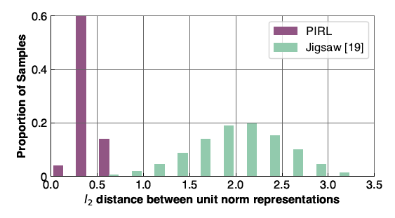
In order to show that the image representations obtained using PIRL are invariant, several images are chosen from ImageNet dataset and representations of the chosen images and their transformed version are obtained using one time PIRL and another time the jigsaw pretext task which is the transformation covariant version of PIRL. Then, for each method, the L2 norm between the original and transformed image representations are computed and their distributions are plotted in Figure (7). It can be seen that PIRL results in more similarity between the original and transformed | In order to show that the image representations obtained using PIRL are invariant, several images are chosen from the ImageNet dataset, and representations of the chosen images and their transformed version are obtained using one-time PIRL and another time the jigsaw pretext task which is the transformation covariant version of PIRL. Then, for each method, the L2 norm between the original and transformed image representations are computed and their distributions are plotted in Figure (7). It can be seen that PIRL results in more similarity between the original and transformed image representations. Therefore, PIRL learns invariant representations. | ||
[[File: SSL_7.PNG | 800px | center]] | [[File: SSL_7.PNG | 800px | center]] | ||
<div align="center">'''Figure 7:''' Invariance of PIRL representations. </div> | <div align="center">'''Figure 7:''' Invariance of PIRL representations. </div> | ||
===Which layer produces the best representation?=== | |||
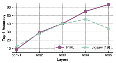
Figure 12 studies the quality of representations in earlier layers of the convolutional networks. The figure reveals that the quality of Jigsaw representations improves from the conv1 to the res4 layer but that their quality sharply decreases in the res5 layer. By contrast, PIRL representations are invariant to image transformations and the best image representations are extracted from the res5 layer of PIRL-trained networks. | |||
[[File: Paper29_SSL.PNG | 800px | center]] | |||
<div align="center">'''Figure 12:'''Quality of PIRL representations per layer. </div> | |||
===What is the effect of <math>\lambda</math> in the PIRL loss function?=== | ===What is the effect of <math>\lambda</math> in the PIRL loss function?=== | ||
| Line 99: | Line 110: | ||
<div align="center">'''Figure 8:''' Effect of varying the parameter <math>\lambda</math> </div> | <div align="center">'''Figure 8:''' Effect of varying the parameter <math>\lambda</math> </div> | ||
===What is the effect of the number of | ===What is the effect of the number of images transforms?=== | ||
As another experiment, the authors investigated the number of image transforms and | As another experiment, the authors investigated the number of image transforms and their effect on PIRL performance. There is a limitation on the number of transformations that can be applied using the jigsaw pretext method as this method has to predict the permutation of the patches and the number of the parameters in the classification layer grows linearly with the number of used transformations. However, PIRL can use all number of image transformations which is equal to <math>9! \approx 3.6\times 10^5</math>. Figure (9) shows the effect of changing the number of patch permutations on PIRL and jigsaw. The results show that increasing the number of permutations increases the mean Average Precision (mAP) of PIRL on image classification using the VOCC07 dataset. | ||
[[File: SSL_9.PNG | 800px | center]] | [[File: SSL_9.PNG | 800px | center]] | ||
| Line 108: | Line 119: | ||
===What is the effect of the number of negative samples?=== | ===What is the effect of the number of negative samples?=== | ||
In order to investigate the effect of negative samples number, N, on PIRL's performance, the image classification accuracy is obtained using ImageNet dataset for a variety of values for N. As it is shown in Figure | In order to investigate the effect of negative samples number, N, on PIRL's performance, the image classification accuracy is obtained using ImageNet dataset for a variety of values for N. As it is shown in Figure 10, increasing the number of negative sample results in richer image representations and higher classification accuracy. | ||
[[File: SSL_10.PNG | 800px | center]] | [[File: SSL_10.PNG | 800px | center]] | ||
| Line 115: | Line 126: | ||
==Generalizing PIRL to Other Pretext Tasks== | ==Generalizing PIRL to Other Pretext Tasks== | ||
The used PIRL model in this paper used jigsaw permutations as the transformation | The used PIRL model in this paper used jigsaw permutations as the applied transformation to the original image. However, PIRL is generalizable to other Pretext Tasks. To show this, first, PIRL is used with rotation transformations and the performance of rotation-based PIRL is compared to the covariant rotation Pretext Task. The results in Figure (11) show that using PIRL substantially increases the classification accuracy on four datasets in comparison with the rotation Pretext Task. Next, both jigsaw and rotation transformations are used with PIRL to obtain image representations. The results show that combining multiple transformations with PIRL can further improve the accuracy of the image classification task. | ||
[[File: SSL_11.PNG | 800px | center]] | [[File: SSL_11.PNG | 800px | center]] | ||
| Line 122: | Line 133: | ||
==Conclusion== | ==Conclusion== | ||
In this paper, a new state-of-the-art Self-Supervised learning method, PIRL, was presented. The proposed model learns to obtain features that are common between the original and transformed images, resulting in a set of transformation invariant and more semantically meaningful features. This is done by defining a contrastive loss function between the original images, transformed images and a set of negative images. The results show that PIRL image representation is richer than previously proposed methods, resulting in higher accuracy and precision on image classification and object detection tasks. | In this paper, a new state-of-the-art Self-Supervised learning method, PIRL, was presented. The proposed model learns to obtain features that are common between the original and transformed images, resulting in a set of transformation invariant and more semantically meaningful features. This is done by defining a contrastive loss function between the original images, transformed images, and a set of negative images. The results show that PIRL image representation is richer than previously proposed methods, resulting in higher accuracy and precision on image classification and object detection tasks. | ||
==Critiques== | |||
The paper proposes a very nice method for obtaining transformation invariant image representations. However, the authors can extend their work with a richer set of transformations. Also, it would be a good idea to investigate the combination of PIRL with clustering-based methods [7,8]. One of the clustering-based methods is '''DeepCluster''' [7], where each previous version of its representation is used by bootstrapping to produce a target for the next representation. They built a new representation through clustering data points using the prior representation and then classify the target by using the clustered index of each sample. That may result in better image representations. This will avoid the use of negative pairs but it might also cause collapsing to trivial solutions which create a trade-off. | |||
It could be better if they could visualize their network weights and compare them to the other supervised methods for the deeper layers that extract high-level information. | |||
== Source Code == | == Source Code == | ||
| Line 130: | Line 147: | ||
== References == | == References == | ||
[1] | [1] Olga Russakovsky, Jia Deng, Hao Su, Jonathan Krause, Sanjeev Satheesh, Sean Ma, Zhiheng Huang, Andrej Karpathy, Aditya Khosla, Michael Bernstein, Alexander C. Berg, and Li Fei-Fei. ImageNet Large Scale Visual Recognition Challenge. IJCV, 2015. | ||
[2] M. Everingham, S. M. A. Eslami, L. Van Gool, C. K. I. Williams, J. Winn, and A. Zisserman. The pascal visual object classes challenge: A retrospective. IJCV, 2015. | |||
[3] Grant Van Horn and Pietro Perona. The devil is in the tails: Fine-grained classification in the wild. arXiv preprint, 2017 | |||
[4] Spyros Gidaris, Praveer Singh, and Nikos Komodakis. Unsupervised representation learning by predicting image rotations. arXiv preprint arXiv:1803.07728, 2018. | |||
[5] Mehdi Noroozi and Paolo Favaro. Unsupervised learning of visual representations by solving jigsaw puzzles. In ECCV, 2016. | |||
[6] Jong-Chyi Su, Subhransu Maji, Bharath Hariharan. When does self-supervision improve few-shot learning? European Conference on Computer Vision, 2020. | |||
[7] Mathilde Caron, Piotr Bojanowski, Armand Joulin, and Matthijs Douze. Deep clustering for unsupervised learning of visual features. In ECCV, 2018. | |||
[8] Mathilde Caron, Piotr Bojanowski, Julien Mairal, and Armand Joulin. Unsupervised pre-training of image features on non-curated data. In ICCV, 2019. | |||
[9] Zhirong Wu, Yuanjun Xiong, Stella X Yu, and Dahua Lin. Unsupervised feature learning via non-parametric instance discrimination. In CVPR, 2018. | |||
Latest revision as of 22:02, 12 December 2020
Authors
Ishan Misra, Laurens van der Maaten
Presented by
Sina Farsangi
Introduction
Modern image recognition and object detection systems find image representations by using a large number of data points with pre-defined semantic annotations. Examples of these annotations include class labels [1] and bounding boxes [2], as shown in Figure 1. There is a need for a large amount of labeled data, which is often very difficult to obtain. Also, these systems usually learn specific features for a particular type of class and not necessarily semantically meaningful features that can help generalize to other domains and classes. In other words, pre-defined semantic annotations scale poorly to the long tail of visual concepts[3]. Therefore, there has been a big interest in the community for learning image representations that are more visually meaningful and can help in a variety of tasks, such as image recognition and object detection. One of the fast-growing areas of research that tries to address this problem is self-supervised Learning. Self-Supervised Learning tries to learn meaningful semantics by just using the inputs themselves rather than using pre-defined semantic annotated data. As will show, the self-supervised learning paradigm removes the need for using human-provided class labels or bounding boxes for classification and object detection tasks, respectively.
Self-Supervised Learning is often done using a set of tasks called pretext tasks. During these tasks, a transformation [math]\displaystyle{ \tau }[/math] is applied to unlabeled images [math]\displaystyle{ I }[/math] to obtain a set of transformed images, [math]\displaystyle{ I^{t} }[/math]. Then, a deep neural network, [math]\displaystyle{ \phi(\theta) }[/math], is trained to predict some characteristic of the transformation from the transformed image. Several pretext tasks exist based on the type of transformation used. For example, if a neural network can accurately determine if an image is upside down or not, then perhaps it has learned some semantically meaningful representation of the image. This pre-empts the need for human-provided labels. Two of the most common pretext tasks used are rotations and jigsaw puzzle [4,5,6]. As shown in Figure 2, in the rotation task, unlabeled images, [math]\displaystyle{ }[/math] are rotated by random degrees (0,90,180,270) and the deep network learns to predict the rotation degree. The jigsaw task is more complicated than the rotation prediction task; first unlabeled images are cropped into 9 patches, then the image is perturbed by randomly permuting the nine patches. The unlabeled original image is referred to as the anchor data point (Figure 3-a), the reshuffled image that we get by permuting patches will be our positive sample (Figure 3-b) and the rest of the images in the dataset will be considered as negative samples. Each permutation falls into one of the 35 classes according to a formula given by the authors. A deep network is then trained to predict the class of the permutation of the patches in the perturbed image. Some other tasks include colorization, where the model tries to revert the colors of a colored image turned to grayscale, and image reconstruction where a square chunk of the image is deleted and the model tries to reconstruct that part.

Although the proposed pretext tasks have achieved promising results, they have the disadvantage of being covariant to the applied transformation. In other words, as deep networks are trained to predict transformation characteristics, they will also learn representations that will vary based on the applied transformation. By intuition, we would like to obtain representations that are common between the original images and the transformed ones. This idea is supported by the fact that humans can recognize these transformed images. For example, a human can identify a permuted image of a tiger (as in figure 3) as a "permuted tiger" as well as the original image as a "tiger". Thus, the "tiger" aspect of the representations human learn is invariant to the transform, which cannot be taken for granted in standard self-supervision. The paper tries to address this problem by introducing Pretext Invariant Representation Learning (PIRL) that obtains representations which are transformation invariant and therefore more semantically meaningful. The performance of the proposed method is evaluated on several self-supervision learning benchmarks. The results show that the PIRL introduces a new state-of-the-art method in self-supervised Learning by learning transformation invariant representations.
Problem Formulation and Methodology
An overview of the proposed method and a comparison with Pretext Tasks are shown in Figure 3. For a given image , [math]\displaystyle{ I }[/math], in the dataset of unlabeled images, [math]\displaystyle{ D=\{{I_1,I_2,...,I_{|D|}}\} }[/math], a transformation [math]\displaystyle{ \tau }[/math] is applied:
\begin{align} \tag{1} \label{eqn:1} I^t=\tau(I) \end{align}
Where [math]\displaystyle{ I^t }[/math] is the transformed image. We would like to train a convolutional neural network, [math]\displaystyle{ \phi(\theta) }[/math], that constructs image representations [math]\displaystyle{ v_{I}=\phi_{\theta}(I) }[/math]. Pretext Task based methods learn to predict transformation characteristics, [math]\displaystyle{ z(t) }[/math], by minimizing a transformation covariant loss function in the form of:
\begin{align} \tag{2} \label{eqn:2} l_{\text{cov}}(\theta,D)=\frac{1}{|D|} \sum_{I \in {D}}^{} L(v_I,z(t)) \end{align}
As it can be seen, the loss function covaries with the applied transformation and therefore, the obtained representations may not be semantically meaningful. PIRL tries to solve for this problem as shown in Figure 3. The original and transformed images are passed through two parallel convolutional neural networks to obtain two sets of representations, [math]\displaystyle{ v(I) }[/math] and [math]\displaystyle{ v(I^t) }[/math]. Then, a contrastive loss function is defined to ensure that the representations of the original and transformed images are similar to each other. The transformation invariant loss function can be defined as:
\begin{align} \tag{3} \label{eqn:3} l_{\text{inv}}(\theta,D)=\frac{1}{|D|} \sum_{I \in {D}}^{} L(v_I,v_{I^t}) \end{align}
Where L is a contrastive loss based on Noise Contrastive Estimators (NCE). The NCE function can be shown as below:
\begin{align} \tag{4} \label{eqn:4} h(v_I,v_{I^t})=\frac{\exp \biggl( \frac{s(v_I,v_{I^t})}{\tau} \biggr)}{\exp \biggl(\frac{s(v_I,v_{I^t})}{\tau} \biggr) + \sum_{I^{'} \in D_N}^{} \exp \biggl( \frac{s(v_{I^t},v_{I^{'}})}{\tau} \biggr)} \end{align}
where [math]\displaystyle{ s(.,.) }[/math] is the cosine similarity function and [math]\displaystyle{ \tau }[/math] is the temperature parameter that is usually set to 0.07. Also, a set of N images are chosen randomly from the dataset where [math]\displaystyle{ I^{'}\neq I }[/math]. These images are used in the loss in order to ensure their representation dissimilarity with transformed image representations. Also, during model implementation, two heads (few additional deep layers), [math]\displaystyle{ f }[/math] and [math]\displaystyle{ g }[/math], are applied on top of [math]\displaystyle{ v(I) }[/math] and [math]\displaystyle{ v(I^t) }[/math]. Using the NCE formulation, the contrastive loss can be written as:
\begin{align} \tag{5} \label{eqn:5} L_{\text{NCE}}(I,I^{t})=-\text{log}[h(f(v_I),g(v_{I^t}))]-\sum_{I^{'}\in D_N}^{} \text{log}[1-h(g(v_{I^t}),f(v_{I^{'}}))] \end{align}
Although the formulation looks complicated, the take-away here is that by minimizing the NCE based loss function, the similarity between the original and transformed image representations, [math]\displaystyle{ v(I) }[/math] and [math]\displaystyle{ v(I^t) }[/math], increases and at the same time the dissimilarity between [math]\displaystyle{ v(I^t) }[/math] and negative images representations, [math]\displaystyle{ v(I^{'}) }[/math], is increased. According to the previous work, an infeasibly large batch size is needed to obtain a large number of negatives. To tackle this problem, a memory bank [9], [math]\displaystyle{ M }[/math], is used during training which contains feature representation [math]\displaystyle{ m_I }[/math] for each image in the dataset including the negative images. The proposed PIRL model is shown in Figure 4. Finally, the contrastive loss in equation \eqref{eqn:5} does not take into account the dissimilarity between the original image representations, [math]\displaystyle{ v(I) }[/math], and the negative image representations, [math]\displaystyle{ v(I^{'}) }[/math]. By taking this into account and using the memory bank, the final contrastive loss function is obtained as:
\begin{align} \tag{6} \label{eqn:6} L(I,I^{t})=\lambda L_{\text{NCE}}(m_I,g(v_{I^t})) + (1-\lambda)L_{\text{NCE}}(m_I,f(v_{I})) \end{align} where [math]\displaystyle{ \lambda }[/math] is a hyperparameter that determines the weight of each of NCE losses. The default value for this parameter is 0.5. In the next section, experimental results are shown using the proposed PIRL model.
Experimental Results
For the experiments in this section, PIRL is implemented using jigsaw transformations. The combination of PIRL with other types of transformations is shown in the last section of the summary. The quality of image representations obtained from PIRL Self-Supervised Learning is evaluated by comparing its performance to other Self-Supervised Learning methods on image recognition and object detection tasks. For the experiments, a ResNet50 model is trained using PIRL and other methods by using 1.28M randomly sampled images from the ImageNet dataset. Also, the number of negative images used for PIRL is N=32000.
Object Detection
A Faster R-CNN model with a ResNet-50 backbone, pre-trained using PIRL and other Self-Supervised methods, is employed for the object detection task. Then, the pre-trained model weights are used as initial weights for the Faster-RCNN model backbone during training on the VOC07+12 dataset. The result of object detection using PIRL is shown in Figure (5) and it is compared to other methods. It can be seen that PIRL not only outperforms other Self-Supervised-based methods, for the first time it outperforms Supervised Pre-training on object detection. They emphasize that PIRL achieves this result using the same backbone model, the same number of finetuning epochs, and the exact same pre-training data (but without the labels). This result is a substantial improvement over prior self-supervised approaches that obtain worse performance than fully supervised baselines despite using orders of magnitude more curated training data or much larger backbone models.
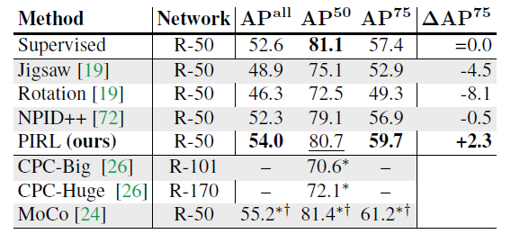
Image Classification with linear models
In the next experiment, the performance of the PIRL is evaluated on image classification using four different datasets. For this experiment, the pre-trained ResNet-50 model is utilized as an image feature extractor. Then, a linear classifier is trained on fixed image representations. The results are shown in Figure (6). The results demonstrate that while PIRL substantially outperforms other Self-Supervised Learning methods, it still falls behind Supervised Pre-trained Learning.
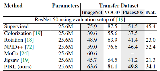
Overall, from Figure6, we can observe that PIRL has the best performance among different Self-Supervised Learning methods. Moreover, PIRL can even perform better than the Supervised Learning Pretrained model on object detection. This is because PIRL learns representations that are invariant to the applied transformations which results in more semantically meaningful and richer visual features. In the next section, some analysis on PIRL is presented.
Analysis
Does PIRL learn invariant representations?
In order to show that the image representations obtained using PIRL are invariant, several images are chosen from the ImageNet dataset, and representations of the chosen images and their transformed version are obtained using one-time PIRL and another time the jigsaw pretext task which is the transformation covariant version of PIRL. Then, for each method, the L2 norm between the original and transformed image representations are computed and their distributions are plotted in Figure (7). It can be seen that PIRL results in more similarity between the original and transformed image representations. Therefore, PIRL learns invariant representations.
Which layer produces the best representation?
Figure 12 studies the quality of representations in earlier layers of the convolutional networks. The figure reveals that the quality of Jigsaw representations improves from the conv1 to the res4 layer but that their quality sharply decreases in the res5 layer. By contrast, PIRL representations are invariant to image transformations and the best image representations are extracted from the res5 layer of PIRL-trained networks.
What is the effect of [math]\displaystyle{ \lambda }[/math] in the PIRL loss function?
In order to investigate the effect of [math]\displaystyle{ \lambda }[/math] on PIRL representations, the authors obtained the accuracy of image recognition on ImageNet dataset using different values for [math]\displaystyle{ \lambda }[/math] in PIRL. As shown in Figure 8, the results show that the value of [math]\displaystyle{ \lambda }[/math] affects the performance of PIRL and the optimum value for [math]\displaystyle{ \lambda }[/math] is 0.5.
What is the effect of the number of images transforms?
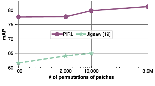
As another experiment, the authors investigated the number of image transforms and their effect on PIRL performance. There is a limitation on the number of transformations that can be applied using the jigsaw pretext method as this method has to predict the permutation of the patches and the number of the parameters in the classification layer grows linearly with the number of used transformations. However, PIRL can use all number of image transformations which is equal to [math]\displaystyle{ 9! \approx 3.6\times 10^5 }[/math]. Figure (9) shows the effect of changing the number of patch permutations on PIRL and jigsaw. The results show that increasing the number of permutations increases the mean Average Precision (mAP) of PIRL on image classification using the VOCC07 dataset.
What is the effect of the number of negative samples?
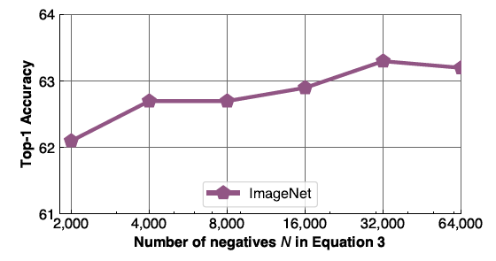
In order to investigate the effect of negative samples number, N, on PIRL's performance, the image classification accuracy is obtained using ImageNet dataset for a variety of values for N. As it is shown in Figure 10, increasing the number of negative sample results in richer image representations and higher classification accuracy.
Generalizing PIRL to Other Pretext Tasks
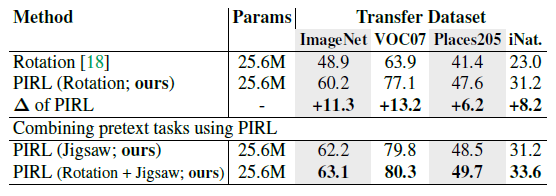
The used PIRL model in this paper used jigsaw permutations as the applied transformation to the original image. However, PIRL is generalizable to other Pretext Tasks. To show this, first, PIRL is used with rotation transformations and the performance of rotation-based PIRL is compared to the covariant rotation Pretext Task. The results in Figure (11) show that using PIRL substantially increases the classification accuracy on four datasets in comparison with the rotation Pretext Task. Next, both jigsaw and rotation transformations are used with PIRL to obtain image representations. The results show that combining multiple transformations with PIRL can further improve the accuracy of the image classification task.
Conclusion
In this paper, a new state-of-the-art Self-Supervised learning method, PIRL, was presented. The proposed model learns to obtain features that are common between the original and transformed images, resulting in a set of transformation invariant and more semantically meaningful features. This is done by defining a contrastive loss function between the original images, transformed images, and a set of negative images. The results show that PIRL image representation is richer than previously proposed methods, resulting in higher accuracy and precision on image classification and object detection tasks.
Critiques
The paper proposes a very nice method for obtaining transformation invariant image representations. However, the authors can extend their work with a richer set of transformations. Also, it would be a good idea to investigate the combination of PIRL with clustering-based methods [7,8]. One of the clustering-based methods is DeepCluster [7], where each previous version of its representation is used by bootstrapping to produce a target for the next representation. They built a new representation through clustering data points using the prior representation and then classify the target by using the clustered index of each sample. That may result in better image representations. This will avoid the use of negative pairs but it might also cause collapsing to trivial solutions which create a trade-off.
It could be better if they could visualize their network weights and compare them to the other supervised methods for the deeper layers that extract high-level information.
Source Code
https://paperswithcode.com/paper/self-supervised-learning-of-pretext-invariant
References
[1] Olga Russakovsky, Jia Deng, Hao Su, Jonathan Krause, Sanjeev Satheesh, Sean Ma, Zhiheng Huang, Andrej Karpathy, Aditya Khosla, Michael Bernstein, Alexander C. Berg, and Li Fei-Fei. ImageNet Large Scale Visual Recognition Challenge. IJCV, 2015.
[2] M. Everingham, S. M. A. Eslami, L. Van Gool, C. K. I. Williams, J. Winn, and A. Zisserman. The pascal visual object classes challenge: A retrospective. IJCV, 2015.
[3] Grant Van Horn and Pietro Perona. The devil is in the tails: Fine-grained classification in the wild. arXiv preprint, 2017
[4] Spyros Gidaris, Praveer Singh, and Nikos Komodakis. Unsupervised representation learning by predicting image rotations. arXiv preprint arXiv:1803.07728, 2018.
[5] Mehdi Noroozi and Paolo Favaro. Unsupervised learning of visual representations by solving jigsaw puzzles. In ECCV, 2016.
[6] Jong-Chyi Su, Subhransu Maji, Bharath Hariharan. When does self-supervision improve few-shot learning? European Conference on Computer Vision, 2020.
[7] Mathilde Caron, Piotr Bojanowski, Armand Joulin, and Matthijs Douze. Deep clustering for unsupervised learning of visual features. In ECCV, 2018.
[8] Mathilde Caron, Piotr Bojanowski, Julien Mairal, and Armand Joulin. Unsupervised pre-training of image features on non-curated data. In ICCV, 2019.
[9] Zhirong Wu, Yuanjun Xiong, Stella X Yu, and Dahua Lin. Unsupervised feature learning via non-parametric instance discrimination. In CVPR, 2018.