MULTI-VIEW DATA GENERATION WITHOUT VIEW SUPERVISION: Difference between revisions
(Created page with "This page contains a summary of the paper "[https://openreview.net/pdf?id=ryRh0bb0Z MULTI-VIEW DATA GENERATION WITHOUT VIEW SUPERVISION]" by Mickael Chen, Ludovic Denoyer, Thi...") |
|||
| (100 intermediate revisions by 19 users not shown) | |||
| Line 1: | Line 1: | ||
This page contains a summary of the paper "[https://openreview.net/ | This page contains a summary of the paper "[https://openreview.net/forum?id=ryRh0bb0Z Multi-View Data Generation without Supervision]" by Mickael Chen, Ludovic Denoyer, Thierry Artieres. It was published at the International Conference on Learning Representations (ICLR) in 2018. An implementation of the models presented in this paper is available here[https://github.com/mickaelChen/GMV] | ||
==Introduction== | ==Introduction== | ||
=== | ===Motivation=== | ||
We are interested in learning generative models that build and make use of a disentangled latent space where the content and the view are encoded separately. We propose to take an original approach by learning such models from multi-view datasets, where (i) samples are labeled based on their content, and without any view information, and (ii) where the generated views are not restricted to be one view in a subset of possible views. High Dimensional Generative models have seen a surge of interest of late with the introduction of Variational Auto-Encoders and Generative Adversarial Networks. This paper focuses on a particular problem where one aims at generating samples corresponding to a number of objects under various views. The distribution of the data is assumed to be driven by two independent latent factors: the content, which represents the intrinsic features of an object, and the view, which stands for the settings of a particular observation of that object (for example, the different angles of the same object). The paper proposes two models using this disentanglement of latent space - a generative model and a conditional variant of the same. The authors claim that unlike many multi-view | |||
approaches, the proposed model doesn’t need any supervision on the views but only on the content. | |||
===Related Work=== | |||
The problem of handling multi-view inputs has mainly been studied from the predictive point of view where one wants, for example, to learn a model able to predict/classify over multiple views of the same object (Su et al. (2015); Qi et al. (2016)). These approaches generally involve (early or late) fusion of the different views at a particular level of a deep architecture. Recent studies have focused on identifying factors of variations from multiview datasets. The underlying idea is to consider that a particular data sample may be thought as the mix of a content information (e.g. related to its class label like a given person in a face dataset) and of a side information, the view, which accounts for factors of variability (e.g. exposure, viewpoint, with/wo glasses...). So, all the samples of the same class contain the same content but different view. A number of approaches have been proposed to disentangle the content from the view (i.e. methods based on unlabeled samples), also referred as the style in some papers (Mathieu et al. (2016); Denton & Birodkar (2017)). The two common limitations the earlier approaches pose - as claimed by the paper - are that (i) they usually | |||
consider discrete views that are characterized by a domain or a set of discrete (binary/categorical) attributes (e.g. face with/wo glasses, the color of the hair, etc.) and could not easily scale to a large number of attributes or to continuous views. (ii) most models are trained using view supervision (e.g. the view attributes), which of course greatly helps in the learning of such model, yet prevents their use on many datasets where this information is not available. | |||
Recently such attempts have been made to learn such models without supervision, but they cannot disentangle high level concepts as only simple features can be reliably captured without any guidance. | |||
===Contributions=== | |||
The contributions that authors claim are the following: (i) A new generative model able to generate data with various content and high view diversity using a supervision on the content information only. (ii) Extend the generative model to a conditional model that allows generating new views over any input sample. (iii) Report experimental results on four different images datasets to prove that the models can generate realistic samples and capture (and generate with) the diversity of views. | |||
Precisely,two models have been proposed: | |||
# a generative model ('''GMV - Generative Multi-view Model''') that generates objects under various views (multiview generation), | |||
# and a conditional extension, '''conditional GMV (C-GMV)''' of this model that generates a large number of views of any input object (conditional multi-view generation). | |||
Both models are based on the adversarial training schema of Generative Adversarial Networks (GAN) proposed in Goodfellow et al. (2014)). The simple but strong idea is to focus on distributions over pairs of examples (e.g. images representing a same object in different views) rather than distribution on single examples. | |||
The | |||
=== | ==Paper Overview== | ||
===Background=== | |||
The paper uses the concept of the popular GAN (Generative Adversarial Networks) proposed by Goodfellow et al.(2014). | |||
GENERATIVE ADVERSARIAL NETWORK: | |||
Generative adversarial networks (GANs) are deep neural net architectures comprised of two nets, pitting one against the other (thus the “adversarial”). GANs was introduced in a paper by Ian Goodfellow and other researchers at the University of Montreal, including Yoshua Bengio, in 2014. Referring to GANs, Facebook’s AI research director Yann LeCun called adversarial training “the most interesting idea in the last 10 years in ML.” | |||
Let us denote <math>X</math> an input space composed of multidimensional samples <math>x</math> e.g. vector, matrix or tensor. Given a latent space <math>R^n</math> and a prior distribution <math>p_z(z)</math> over this latent space, any generator function <math>G : R^n → X</math> defines a distribution <math>p_G </math> on <math> X</math> which is the distribution of samples <math>G(z)</math> where <math>z ∼ p_z</math>. A GAN defines, in addition to <math>G</math>, a discriminator function <math>D : X → [0; 1]</math> which aims at differentiating between real inputs sampled from the training set and fake inputs sampled from <math>p_G</math>, while the generator learns to fool the discriminator <math>D</math>. Usually both <math>G</math> and <math>D</math> are implemented with neural networks. The objective function is based on the following adversarial criterion: | |||
<div style="text-align: center;font-size:100%"><math>\underset{G}{min} \ \underset{D}{max}</math> <math>E_{p_x}[log D(x)] + Ep_z[log(1 − D(G(z)))]</math></div> | |||
where <math>p_x</math> is the empirical data distribution on <math>X</math> . | |||
It has been shown in Goodfellow et al. (2014) that if G∗ and D∗ are optimal for the above criterion, the Jensen-Shannon divergence between <math>p_{G∗}</math> and the empirical distribution of the data <math>p_x</math> in the dataset is minimized, making GAN able to estimate complex continuous data distributions. | |||
CONDITIONAL GENERATIVE ADVERSARIAL NETWORK: | |||
In | In the Conditional GAN (CGAN), the generator learns to generate a fake sample with a specific condition or characteristics (such as a label associated with an image or more detailed tag) rather than a generic sample from unknown noise distribution. The conditionality of a CGAN is determined by defining a generator function <math>G</math> which takes a noise vector <math>z</math> and a condition <math>y</math> as inputs. Now, to add such a condition to both generator and discriminator, we will simply feed some vector <math>y</math>, into both networks. Hence, both the discriminator <math>D(X,y)</math> and generator <math>G(z,y)</math> are jointly distributed with <math>y</math>. A target <math>X</math> from a given input <math>y</math> can be obtained by first sampling the latent vector <math>z ∼ p_z</math>, then by computing <math>G(y, z)</math>. The discriminator takes both the condition <math>y</math> and the datapoint <math>x</math> as inputs. | ||
Now, the objective function of CGAN is: | |||
<div style="text-align: center;font-size:100%"><math>\underset{G}{min} \ \underset{D}{max}</math> <math>E_{p_x}[log D(x,y)] + Ep_z[log(1 − D(G(y,z)))]</math></div> | |||
< | The paper also suggests that many studies have reported that when dealing with high-dimensional input spaces, CGAN tends to collapse the modes of the data distribution, mostly ignoring the latent factor <math>z</math> and generating <math>x</math> only based on the condition <math>y</math>, exhibiting an almost deterministic behavior. At this point, the CGAN also fails to produce a satisfying amount of diversity in generated samples. | ||
===Generative Multi-View Model=== | |||
The | ''' Objective and Notations: ''' The distribution of the data x ∈ X is assumed to be driven by two latent factors: a content factor denoted c which corresponds to the invariant proprieties of the object and a view factor denoted v which corresponds to the factor of variations. Typically, if X is the space of people’s faces, c stands for the intrinsic features of a person’s face while v stands for the transient features and the viewpoint of a particular photo of the face, including the photo exposure | ||
and additional elements like a hat, glasses, etc.... These two factors c and v are assumed to be independent and these are the factors needed to learn. | |||
The paper defines two tasks here to be done: | |||
(i) '''Multi View Generation''': we want to be able to sample over X by controlling the two factors c and v. Given two priors, p(c) and p(v), this sampling will be possible if we are able to estimate p(x|c, v) from a training set. | |||
(ii) '''Conditional Multi-View Generation''': the second objective is to be able to sample different views of a given object. Given a prior p(v), this sampling will be achieved by learning the probability p(c|x), in addition to p(x|c, v). Ability to learn generative models able to generate from a disentangled latent space would allow controlling the sampling on the two different axes, | |||
the content and the view. The authors claim the originality of work is to learn such generative models without using any view labeling information. | |||
The paper introduces the vectors '''c''' and '''v''' to represent latent vectors in R<sup>c</sup> and R<sup>v</sup> | |||
''' Generative Multi-view Model: ''' | |||
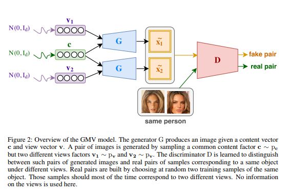
Consider two prior distributions over the content and view factors denoted as <math>p_c</math> and <math>p_v</math>, corresponding to the prior distribution over content and latent factors. Moreover, we consider a generator G that implements a distribution over samples x, denoted as <math>p_G</math> by computing G(c, v) with <math>c ∼ p_c</math> and <math>v ∼ p_v</math>. The objective is to learn this generator so that its first input c corresponds to the content of the generated sample while its second input v, captures the underlying view of the sample. Doing so would allow one to control the output sample of the generator by tuning its content or its view (i.e. c and v). | |||
The key idea that the authors propose is to focus on the distribution of pairs of inputs rather than on the distribution over individual samples. When no view supervision is available the only valuable pairs of samples that one may build from the dataset consist of two samples of a given object under two different views. When we choose any two samples randomly from the dataset from the same object, it is most likely that we get two different views. The paper explains that there are three goals here, (i) As in regular GAN, each sample generated by G needs to look realistic. (ii) As real pairs are composed of two views of the same object, the generator should generate pairs of the same object. Since the two sampled view factors v1 and v2 are different, the only way this can be achieved is by encoding the content vector c which is invariant. (iii) It is expected that the discriminator should easily discriminate between a pair of samples corresponding to the same object under different views from a pair of samples corresponding to a same object under the same view. Because the pair shares the same content factor c, this should force the generator to use the view factors v1 and v2 to produce diversity in the generated pair. | |||
Now, the objective function of GMV Model is: | |||
< | <div style="text-align: center;font-size:100%"><math>\underset{G}{min} \ \underset{D}{max}</math> <math>E_{x_1,x_2}[log D(x_1,x_2)] + E_{v_1,v_2}[log(1 − D(G(c,v_1),G(c,v_2)))]</math></div> | ||
Once the model is learned, generator G that generates single samples by first sampling c and v following <math>p_c</math> and <math>p_v</math>, then by computing G(c, v). By freezing c or v, one may then generate samples corresponding to multiple views of any particular content, or corresponding to many contents under a particular view. One can also make interpolations between two given views over a particular content, or between two contents using a particular view | |||
<div style="text-align: center;font-size:100%">[[File:GMV.png]]</div> | |||
===Conditional Generative Model (C-GMV)=== | |||
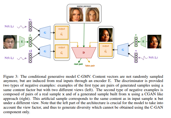
C-GMV is proposed by the authors to be able to change the view of a given object that would be provided as an input to the model. This model extends the generative model's the ability to extract the content factor from any given input and to use this extracted content in order to generate new views of the corresponding object. To achieve such a goal, we must add to our generative model an encoder function denoted <math>E : X → R^C</math> that will map any input in X to the content space <math>R^C</math> | |||
Input sample x is encoded in the content space using an encoder function, noted E (implemented as a neural network). | |||
This encoder serves to generate a content vector c = E(x) that will be combined with a randomly sampled view <math>v ∼ p_v</math> to generate an artificial example. The artificial sample is then combined with the original input x to form a negative pair. The issue with this approach is that CGAN is known to easily miss modes of the underlying distribution. The generator enters in a state where it ignores the noisy component v. To overcome this phenomenon, we use the same idea as in GMV. We build negative pairs <math>(G(c, v_1), G(c, v_2))</math> by randomly sampling two views <math>v_1</math> and <math>v_2</math> that are combined to get a unique content c. c is computed from a sample x using the encoder E, i.e. c= E(x). By doing so, the ability of our approach to generating pairs with view diversity is preserved. Since this diversity can only be captured by taking into account the two different view vectors provided to the model (<math>v_1</math> and <math>v_2</math>), this will encourage G(c, v) to generate samples containing both the content information c, and the view v. Positive pairs are sampled from the training set and correspond to two views of a given object. | |||
< | |||
< | |||
The Objective function for C-GMV will be: | |||
<div style="text-align: center;font-size:100%"><math>\underset{G}{min} \ \underset{D}{max}</math> <math>E_{x_1,x_2 ~ p_x|l(x_1)=l(x_2)}[log D(x_1,x_2)] + E_{v_1,v_2 ~ p_v,x~p_x}[log(1 − D(G(E(x),v_1),G(E(x),v_2)))]+E_{v∼p_v,x∼p_x}[log(1 − D(G(E(x), v), x))] </math></div> | |||
<div style="text-align: center;font-size:100%"> | <div style="text-align: center;font-size:100%">[[File:CGMV.png]]</div> | ||
At inference time, as with the GMV model, we are interested in getting the encoder E and the | |||
generator G. These models may be used for generating new views of any object which is observed | |||
as an input sample x by computing its content vector E(x), then sampling <math>v ∼ p_v</math> and finally by | |||
computing the output G(E(x), v) | |||
==Experiments and Results== | |||
The authors have given an exhaustive set of results and experiments. | |||
The | Datasets: The two models were evaluated by performing experiments over four image datasets of various domains. Note that when supervision is available on the views (like CelebA for example where images are labeled with attributes) it is not used for learning models. The only supervision that is used is if two samples correspond to the same object or not. | ||
<div style="text-align: center;font-size:100%">[[File:table_data.png]]</div> | |||
The | Model Architecture: Same architectures for every dataset. The images were rescaled to 3×64×64 tensors. The generator G and the discriminator D follow that of the DCGAN implementation proposed in Radford et al. (2015). The encoder E is similar to D with the only differences being the batch-normalization in the first layer and the last layer which doesn't have a non-linearity. The Adam optimizer was used, with a batch size of 128. The learning rates for G and D were set to 1*10<sup>-3</sup> and 2*10<sup>-4</sup> respectively for the GMV experiments. In the C-GMV experiments, learning rates of 5*10<sup>-5</sup> were used. Alternating gradient descent was used to optimize the different objectives of the network components (generator, encoder and discriminator). | ||
Baselines: Most existing methods are learned on datasets with view labeling. To fairly compare with alternative models, authors have built baselines working in the same conditions as the models in this paper. In addition, models are compared with the model from Mathieu et al. (2016). Results gained with two implementations are reported, the first one based on the implementation provided by the authors2 (denoted Mathieu et al. (2016)), and the second one (denoted Mathieu et al. (2016) (DCGAN) ) that implements the same model using architectures inspired from DCGAN Radford et al. (2015), which is more stable and that was tuned to allow a fair comparison with our approach. For pure multi-view generative setting, generative model(GMV) is compared with standard GANs that are learned to approximate the joint generation of multiple samples: DCGANx2 is learned to output pairs of views over the same object, DCGANx4 is trained on quadruplets, and DCGANx8 on eight different views. | |||
===Generating Multiple Contents and Views=== | |||
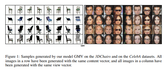
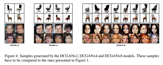
Figure 1 shows examples of generated images by our model and Figure 4 shows images sampled by the DCGAN based models (DCGANx2, DCGANx4, and DCGANx8) on 3DChairs and CelebA datasets. | |||
<div style="text-align: center;font-size:100%">[[File:fig1_gmv.png]]</div> | |||
= | <div style="text-align: center;font-size:100%">[[File:fig4_gmv.png]]</div> | ||
Figure 5 shows additional results, using the same presentation, for the GMV model only on two other datasets. In the left hand block of Figure 5, each row shows different views generated given the same content. | |||
<div style="text-align: center;font-size:100%">[[File:fig5_gmv.png]]</div> | |||
Figure 6 shows generated samples obtained by interpolation between two different view factors (left) or two content factors (right). Again, in the left and right hand block of Figure 6, each row shows different views generated given the same content. It allows us to have a better idea of the underlying view/content structure captured by GMV. We can see that our approach is able to smoothly move from one content/view to another content/view while keeping the other factor constant. This also illustrates that content and view factors are well independently handled by the generator i.e. changing the view | |||
does not modify the content and vice versa. | |||
<div style="text-align: center;font-size:100%">[[File:fig6_gmv.png]]</div> | |||
===Generating Multiple Views of a Given Object=== | |||
The second set of experiments evaluates the ability of C-GMV to capture a particular content from an input sample and to use this content to generate multiple views of the same object. Figure 7 and 8 illustrate the diversity of views in samples generated by our model and compare our results with those obtained with the CGAN model and to models from Mathieu et al. (2016). For each row, the input sample is shown in the left column. New views are generated from that input and shown to the right, with those generated from C_GMV in the centre, and those generated from CGAN on the far right. | |||
[[File: | <div style="text-align: center;font-size:100%">[[File:fig7_gmv.png]]</div> | ||
<div style="text-align: center;font-size:100%">[[File:fig8_gmv.png]]</div> | |||
=== Evaluation of the Quality of Generated Samples === | |||
There are usually several metrics to evaluate generative models. Some of them are: | |||
( | <ol> | ||
<li>Inception Score: In a general sense, the Inception Score is a metric used to quantify the “realness” of a generated image. It is calculated across a set of generated images, and considers two criteria. First, all images of the sample class should be similar (low in-class variance). And second, the distribution of classes should not be dominated by any particular class. The better these criteria are met; the higher the Inception Score.</li> | |||
<li>Latent Space Interpolation</li> | |||
<li>log-likelihood (LL) score</li> | |||
<li> minimum description length (MDL) score</li> | |||
<li>minimum message length (MML) score</li> | |||
<li>Akaike Information Criterion (AIC) score</li> | |||
<li>Bayesian Information Criterion (BIC) score</li> | |||
</ol> | |||
The authors did sets of experiments aimed at evaluating the quality of the generated samples. They have been made on the CelebA dataset and evaluate (i) the ability of the models to preserve the identity of a person in multiple generated views, (ii) to generate realistic samples, (iii) to preserve the diversity in the generated views and (iv) to capture the view distributions of the original dataset. | |||
<div style="text-align: center;font-size:100%">[[File:tab3.png]]</div> | |||
<div style="text-align: center;font-size:100%">[[File:tab4.png]]</div> | |||
= | <div style="text-align: center;font-size:100%">[[File:table.png]]</div> | ||
==Conclusion== | |||
The paper proposed a generative model, which can be learnt from multi-view data without any supervision. Moreover, it introduced a conditional version that allows generating new views of an input image. Using experiments, they proved that the model can capture content and view factors. Here, the paper showed that the application of architecture search to dense image prediction was achieved through a) The construction of a recursive search space leveraging innovation in the dense prediction literature b) construction of a fast proxy predictive of a large task. The learned architecture was shown to surpass human invented architectures across three dense image prediction tasks i.e scene parsing, person part segmentation and semantic segmentation. In the future, they are planning to use the method of this paper for data augmentation which can enrich training dataset. . | |||
The | ==Future Work== | ||
The authors of the papers mentioned that they plan to explore using their model for data augmentation, as it can produce other data views for training, in both semi-supervised and one-shot/few-shot learning settings. | |||
==Critique== | |||
The main idea is to train the model with pairs of images with different views. It is not that clear as to what defines a view in particular. The algorithms are largely based on earlier concepts of GAN and CGAN The authors give reference to the previous papers tackling the same problem and clearly define that the novelty in this approach is not making use of view labels. The authors give a very thorough list of experiments which clearly establish the superiority of the proposed models to baselines. | |||
However, this paper only tested the model on rather constrained examples. As was observed in the results the proposed approach seems to have a high sample complexity relying on training samples covering the full range of variations for both specified and unspecified variations. Also, the proposed model does not attempt to disentangle variations within the specified and unspecified components. | |||
The method that the paper presented is novel and the paper is easy to follow. However, the authors only show a comparison between the proposed method and several baselines: DCGAN and CGAN and do not compare with the methods from Mathieu et al. 2016. In addition, the experiment result is empirical, we do not know the performance of this method in practice in the real world. | |||
==References== | |||
[ | [1] Mickael Chen, Ludovic Denoyer, Thierry Artieres. MULTI-VIEW DATA GENERATION WITHOUT VIEW SUPERVISION. Published as a conference paper at ICLR 2018 | ||
[ | [2] Michael F Mathieu, Junbo Jake Zhao, Junbo Zhao, Aditya Ramesh, Pablo Sprechmann, and Yann LeCun. Disentangling factors of variation in deep representation using adversarial training. In Advances in Neural Information Processing Systems, pp. 5040–5048, 2016. | ||
[ | [3] Mathieu Aubry, Daniel Maturana, Alexei Efros, Bryan Russell, and Josef Sivic. Seeing 3d chairs: exemplar part-based 2d-3d alignment using a large dataset of cad models. In CVPR, 2014. | ||
[ | [4] Ian Goodfellow, Jean Pouget-Abadie, Mehdi Mirza, Bing Xu, David Warde-Farley, Sherjil Ozair, Aaron Courville, and Yoshua Bengio. Generative adversarial nets. In Advances in neural information processing systems, pp. 2672–2680, 2014. | ||
[ | [5] Emily Denton and Vighnesh Birodkar. Unsupervised learning of disentangled representations from video. arXiv preprint arXiv:1705.10915, 2017. | ||
Latest revision as of 00:34, 14 December 2018
This page contains a summary of the paper "Multi-View Data Generation without Supervision" by Mickael Chen, Ludovic Denoyer, Thierry Artieres. It was published at the International Conference on Learning Representations (ICLR) in 2018. An implementation of the models presented in this paper is available here[1]
Introduction
Motivation
We are interested in learning generative models that build and make use of a disentangled latent space where the content and the view are encoded separately. We propose to take an original approach by learning such models from multi-view datasets, where (i) samples are labeled based on their content, and without any view information, and (ii) where the generated views are not restricted to be one view in a subset of possible views. High Dimensional Generative models have seen a surge of interest of late with the introduction of Variational Auto-Encoders and Generative Adversarial Networks. This paper focuses on a particular problem where one aims at generating samples corresponding to a number of objects under various views. The distribution of the data is assumed to be driven by two independent latent factors: the content, which represents the intrinsic features of an object, and the view, which stands for the settings of a particular observation of that object (for example, the different angles of the same object). The paper proposes two models using this disentanglement of latent space - a generative model and a conditional variant of the same. The authors claim that unlike many multi-view approaches, the proposed model doesn’t need any supervision on the views but only on the content.
Related Work
The problem of handling multi-view inputs has mainly been studied from the predictive point of view where one wants, for example, to learn a model able to predict/classify over multiple views of the same object (Su et al. (2015); Qi et al. (2016)). These approaches generally involve (early or late) fusion of the different views at a particular level of a deep architecture. Recent studies have focused on identifying factors of variations from multiview datasets. The underlying idea is to consider that a particular data sample may be thought as the mix of a content information (e.g. related to its class label like a given person in a face dataset) and of a side information, the view, which accounts for factors of variability (e.g. exposure, viewpoint, with/wo glasses...). So, all the samples of the same class contain the same content but different view. A number of approaches have been proposed to disentangle the content from the view (i.e. methods based on unlabeled samples), also referred as the style in some papers (Mathieu et al. (2016); Denton & Birodkar (2017)). The two common limitations the earlier approaches pose - as claimed by the paper - are that (i) they usually consider discrete views that are characterized by a domain or a set of discrete (binary/categorical) attributes (e.g. face with/wo glasses, the color of the hair, etc.) and could not easily scale to a large number of attributes or to continuous views. (ii) most models are trained using view supervision (e.g. the view attributes), which of course greatly helps in the learning of such model, yet prevents their use on many datasets where this information is not available.
Recently such attempts have been made to learn such models without supervision, but they cannot disentangle high level concepts as only simple features can be reliably captured without any guidance.
Contributions
The contributions that authors claim are the following: (i) A new generative model able to generate data with various content and high view diversity using a supervision on the content information only. (ii) Extend the generative model to a conditional model that allows generating new views over any input sample. (iii) Report experimental results on four different images datasets to prove that the models can generate realistic samples and capture (and generate with) the diversity of views.
Precisely,two models have been proposed:
- a generative model (GMV - Generative Multi-view Model) that generates objects under various views (multiview generation),
- and a conditional extension, conditional GMV (C-GMV) of this model that generates a large number of views of any input object (conditional multi-view generation).
Both models are based on the adversarial training schema of Generative Adversarial Networks (GAN) proposed in Goodfellow et al. (2014)). The simple but strong idea is to focus on distributions over pairs of examples (e.g. images representing a same object in different views) rather than distribution on single examples.
Paper Overview
Background
The paper uses the concept of the popular GAN (Generative Adversarial Networks) proposed by Goodfellow et al.(2014).
GENERATIVE ADVERSARIAL NETWORK:
Generative adversarial networks (GANs) are deep neural net architectures comprised of two nets, pitting one against the other (thus the “adversarial”). GANs was introduced in a paper by Ian Goodfellow and other researchers at the University of Montreal, including Yoshua Bengio, in 2014. Referring to GANs, Facebook’s AI research director Yann LeCun called adversarial training “the most interesting idea in the last 10 years in ML.”
Let us denote [math]\displaystyle{ X }[/math] an input space composed of multidimensional samples [math]\displaystyle{ x }[/math] e.g. vector, matrix or tensor. Given a latent space [math]\displaystyle{ R^n }[/math] and a prior distribution [math]\displaystyle{ p_z(z) }[/math] over this latent space, any generator function [math]\displaystyle{ G : R^n → X }[/math] defines a distribution [math]\displaystyle{ p_G }[/math] on [math]\displaystyle{ X }[/math] which is the distribution of samples [math]\displaystyle{ G(z) }[/math] where [math]\displaystyle{ z ∼ p_z }[/math]. A GAN defines, in addition to [math]\displaystyle{ G }[/math], a discriminator function [math]\displaystyle{ D : X → [0; 1] }[/math] which aims at differentiating between real inputs sampled from the training set and fake inputs sampled from [math]\displaystyle{ p_G }[/math], while the generator learns to fool the discriminator [math]\displaystyle{ D }[/math]. Usually both [math]\displaystyle{ G }[/math] and [math]\displaystyle{ D }[/math] are implemented with neural networks. The objective function is based on the following adversarial criterion:
where [math]\displaystyle{ p_x }[/math] is the empirical data distribution on [math]\displaystyle{ X }[/math] . It has been shown in Goodfellow et al. (2014) that if G∗ and D∗ are optimal for the above criterion, the Jensen-Shannon divergence between [math]\displaystyle{ p_{G∗} }[/math] and the empirical distribution of the data [math]\displaystyle{ p_x }[/math] in the dataset is minimized, making GAN able to estimate complex continuous data distributions.
CONDITIONAL GENERATIVE ADVERSARIAL NETWORK:
In the Conditional GAN (CGAN), the generator learns to generate a fake sample with a specific condition or characteristics (such as a label associated with an image or more detailed tag) rather than a generic sample from unknown noise distribution. The conditionality of a CGAN is determined by defining a generator function [math]\displaystyle{ G }[/math] which takes a noise vector [math]\displaystyle{ z }[/math] and a condition [math]\displaystyle{ y }[/math] as inputs. Now, to add such a condition to both generator and discriminator, we will simply feed some vector [math]\displaystyle{ y }[/math], into both networks. Hence, both the discriminator [math]\displaystyle{ D(X,y) }[/math] and generator [math]\displaystyle{ G(z,y) }[/math] are jointly distributed with [math]\displaystyle{ y }[/math]. A target [math]\displaystyle{ X }[/math] from a given input [math]\displaystyle{ y }[/math] can be obtained by first sampling the latent vector [math]\displaystyle{ z ∼ p_z }[/math], then by computing [math]\displaystyle{ G(y, z) }[/math]. The discriminator takes both the condition [math]\displaystyle{ y }[/math] and the datapoint [math]\displaystyle{ x }[/math] as inputs.
Now, the objective function of CGAN is:
The paper also suggests that many studies have reported that when dealing with high-dimensional input spaces, CGAN tends to collapse the modes of the data distribution, mostly ignoring the latent factor [math]\displaystyle{ z }[/math] and generating [math]\displaystyle{ x }[/math] only based on the condition [math]\displaystyle{ y }[/math], exhibiting an almost deterministic behavior. At this point, the CGAN also fails to produce a satisfying amount of diversity in generated samples.
Generative Multi-View Model
Objective and Notations: The distribution of the data x ∈ X is assumed to be driven by two latent factors: a content factor denoted c which corresponds to the invariant proprieties of the object and a view factor denoted v which corresponds to the factor of variations. Typically, if X is the space of people’s faces, c stands for the intrinsic features of a person’s face while v stands for the transient features and the viewpoint of a particular photo of the face, including the photo exposure and additional elements like a hat, glasses, etc.... These two factors c and v are assumed to be independent and these are the factors needed to learn.
The paper defines two tasks here to be done: (i) Multi View Generation: we want to be able to sample over X by controlling the two factors c and v. Given two priors, p(c) and p(v), this sampling will be possible if we are able to estimate p(x|c, v) from a training set. (ii) Conditional Multi-View Generation: the second objective is to be able to sample different views of a given object. Given a prior p(v), this sampling will be achieved by learning the probability p(c|x), in addition to p(x|c, v). Ability to learn generative models able to generate from a disentangled latent space would allow controlling the sampling on the two different axes, the content and the view. The authors claim the originality of work is to learn such generative models without using any view labeling information.
The paper introduces the vectors c and v to represent latent vectors in Rc and Rv
Generative Multi-view Model:
Consider two prior distributions over the content and view factors denoted as [math]\displaystyle{ p_c }[/math] and [math]\displaystyle{ p_v }[/math], corresponding to the prior distribution over content and latent factors. Moreover, we consider a generator G that implements a distribution over samples x, denoted as [math]\displaystyle{ p_G }[/math] by computing G(c, v) with [math]\displaystyle{ c ∼ p_c }[/math] and [math]\displaystyle{ v ∼ p_v }[/math]. The objective is to learn this generator so that its first input c corresponds to the content of the generated sample while its second input v, captures the underlying view of the sample. Doing so would allow one to control the output sample of the generator by tuning its content or its view (i.e. c and v).
The key idea that the authors propose is to focus on the distribution of pairs of inputs rather than on the distribution over individual samples. When no view supervision is available the only valuable pairs of samples that one may build from the dataset consist of two samples of a given object under two different views. When we choose any two samples randomly from the dataset from the same object, it is most likely that we get two different views. The paper explains that there are three goals here, (i) As in regular GAN, each sample generated by G needs to look realistic. (ii) As real pairs are composed of two views of the same object, the generator should generate pairs of the same object. Since the two sampled view factors v1 and v2 are different, the only way this can be achieved is by encoding the content vector c which is invariant. (iii) It is expected that the discriminator should easily discriminate between a pair of samples corresponding to the same object under different views from a pair of samples corresponding to a same object under the same view. Because the pair shares the same content factor c, this should force the generator to use the view factors v1 and v2 to produce diversity in the generated pair.
Now, the objective function of GMV Model is:
Once the model is learned, generator G that generates single samples by first sampling c and v following [math]\displaystyle{ p_c }[/math] and [math]\displaystyle{ p_v }[/math], then by computing G(c, v). By freezing c or v, one may then generate samples corresponding to multiple views of any particular content, or corresponding to many contents under a particular view. One can also make interpolations between two given views over a particular content, or between two contents using a particular view
Conditional Generative Model (C-GMV)
C-GMV is proposed by the authors to be able to change the view of a given object that would be provided as an input to the model. This model extends the generative model's the ability to extract the content factor from any given input and to use this extracted content in order to generate new views of the corresponding object. To achieve such a goal, we must add to our generative model an encoder function denoted [math]\displaystyle{ E : X → R^C }[/math] that will map any input in X to the content space [math]\displaystyle{ R^C }[/math]
Input sample x is encoded in the content space using an encoder function, noted E (implemented as a neural network). This encoder serves to generate a content vector c = E(x) that will be combined with a randomly sampled view [math]\displaystyle{ v ∼ p_v }[/math] to generate an artificial example. The artificial sample is then combined with the original input x to form a negative pair. The issue with this approach is that CGAN is known to easily miss modes of the underlying distribution. The generator enters in a state where it ignores the noisy component v. To overcome this phenomenon, we use the same idea as in GMV. We build negative pairs [math]\displaystyle{ (G(c, v_1), G(c, v_2)) }[/math] by randomly sampling two views [math]\displaystyle{ v_1 }[/math] and [math]\displaystyle{ v_2 }[/math] that are combined to get a unique content c. c is computed from a sample x using the encoder E, i.e. c= E(x). By doing so, the ability of our approach to generating pairs with view diversity is preserved. Since this diversity can only be captured by taking into account the two different view vectors provided to the model ([math]\displaystyle{ v_1 }[/math] and [math]\displaystyle{ v_2 }[/math]), this will encourage G(c, v) to generate samples containing both the content information c, and the view v. Positive pairs are sampled from the training set and correspond to two views of a given object.
The Objective function for C-GMV will be:
At inference time, as with the GMV model, we are interested in getting the encoder E and the
generator G. These models may be used for generating new views of any object which is observed
as an input sample x by computing its content vector E(x), then sampling [math]\displaystyle{ v ∼ p_v }[/math] and finally by
computing the output G(E(x), v)
Experiments and Results
The authors have given an exhaustive set of results and experiments.
Datasets: The two models were evaluated by performing experiments over four image datasets of various domains. Note that when supervision is available on the views (like CelebA for example where images are labeled with attributes) it is not used for learning models. The only supervision that is used is if two samples correspond to the same object or not.
Model Architecture: Same architectures for every dataset. The images were rescaled to 3×64×64 tensors. The generator G and the discriminator D follow that of the DCGAN implementation proposed in Radford et al. (2015). The encoder E is similar to D with the only differences being the batch-normalization in the first layer and the last layer which doesn't have a non-linearity. The Adam optimizer was used, with a batch size of 128. The learning rates for G and D were set to 1*10-3 and 2*10-4 respectively for the GMV experiments. In the C-GMV experiments, learning rates of 5*10-5 were used. Alternating gradient descent was used to optimize the different objectives of the network components (generator, encoder and discriminator).
Baselines: Most existing methods are learned on datasets with view labeling. To fairly compare with alternative models, authors have built baselines working in the same conditions as the models in this paper. In addition, models are compared with the model from Mathieu et al. (2016). Results gained with two implementations are reported, the first one based on the implementation provided by the authors2 (denoted Mathieu et al. (2016)), and the second one (denoted Mathieu et al. (2016) (DCGAN) ) that implements the same model using architectures inspired from DCGAN Radford et al. (2015), which is more stable and that was tuned to allow a fair comparison with our approach. For pure multi-view generative setting, generative model(GMV) is compared with standard GANs that are learned to approximate the joint generation of multiple samples: DCGANx2 is learned to output pairs of views over the same object, DCGANx4 is trained on quadruplets, and DCGANx8 on eight different views.
Generating Multiple Contents and Views
Figure 1 shows examples of generated images by our model and Figure 4 shows images sampled by the DCGAN based models (DCGANx2, DCGANx4, and DCGANx8) on 3DChairs and CelebA datasets.
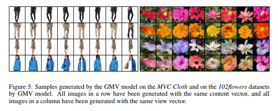
Figure 5 shows additional results, using the same presentation, for the GMV model only on two other datasets. In the left hand block of Figure 5, each row shows different views generated given the same content.
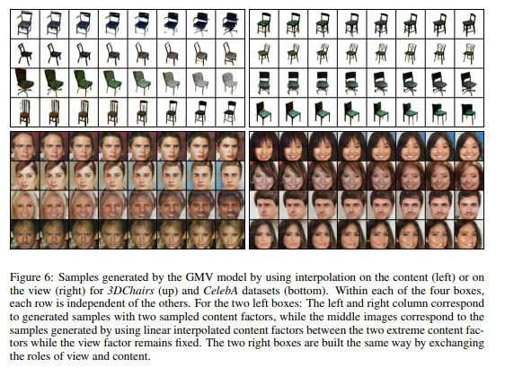
Figure 6 shows generated samples obtained by interpolation between two different view factors (left) or two content factors (right). Again, in the left and right hand block of Figure 6, each row shows different views generated given the same content. It allows us to have a better idea of the underlying view/content structure captured by GMV. We can see that our approach is able to smoothly move from one content/view to another content/view while keeping the other factor constant. This also illustrates that content and view factors are well independently handled by the generator i.e. changing the view does not modify the content and vice versa.
Generating Multiple Views of a Given Object
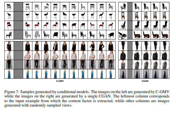
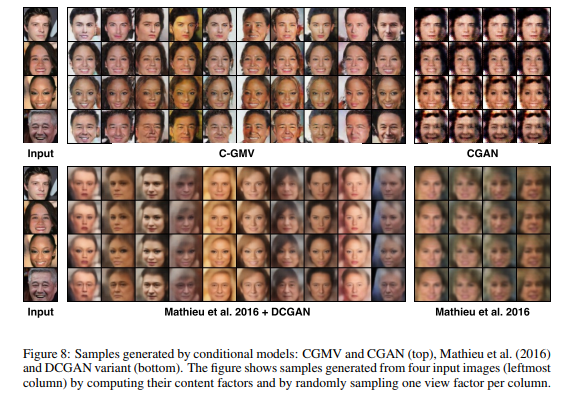
The second set of experiments evaluates the ability of C-GMV to capture a particular content from an input sample and to use this content to generate multiple views of the same object. Figure 7 and 8 illustrate the diversity of views in samples generated by our model and compare our results with those obtained with the CGAN model and to models from Mathieu et al. (2016). For each row, the input sample is shown in the left column. New views are generated from that input and shown to the right, with those generated from C_GMV in the centre, and those generated from CGAN on the far right.
Evaluation of the Quality of Generated Samples
There are usually several metrics to evaluate generative models. Some of them are:
- Inception Score: In a general sense, the Inception Score is a metric used to quantify the “realness” of a generated image. It is calculated across a set of generated images, and considers two criteria. First, all images of the sample class should be similar (low in-class variance). And second, the distribution of classes should not be dominated by any particular class. The better these criteria are met; the higher the Inception Score.
- Latent Space Interpolation
- log-likelihood (LL) score
- minimum description length (MDL) score
- minimum message length (MML) score
- Akaike Information Criterion (AIC) score
- Bayesian Information Criterion (BIC) score
The authors did sets of experiments aimed at evaluating the quality of the generated samples. They have been made on the CelebA dataset and evaluate (i) the ability of the models to preserve the identity of a person in multiple generated views, (ii) to generate realistic samples, (iii) to preserve the diversity in the generated views and (iv) to capture the view distributions of the original dataset.
Conclusion
The paper proposed a generative model, which can be learnt from multi-view data without any supervision. Moreover, it introduced a conditional version that allows generating new views of an input image. Using experiments, they proved that the model can capture content and view factors. Here, the paper showed that the application of architecture search to dense image prediction was achieved through a) The construction of a recursive search space leveraging innovation in the dense prediction literature b) construction of a fast proxy predictive of a large task. The learned architecture was shown to surpass human invented architectures across three dense image prediction tasks i.e scene parsing, person part segmentation and semantic segmentation. In the future, they are planning to use the method of this paper for data augmentation which can enrich training dataset. .
Future Work
The authors of the papers mentioned that they plan to explore using their model for data augmentation, as it can produce other data views for training, in both semi-supervised and one-shot/few-shot learning settings.
Critique
The main idea is to train the model with pairs of images with different views. It is not that clear as to what defines a view in particular. The algorithms are largely based on earlier concepts of GAN and CGAN The authors give reference to the previous papers tackling the same problem and clearly define that the novelty in this approach is not making use of view labels. The authors give a very thorough list of experiments which clearly establish the superiority of the proposed models to baselines.
However, this paper only tested the model on rather constrained examples. As was observed in the results the proposed approach seems to have a high sample complexity relying on training samples covering the full range of variations for both specified and unspecified variations. Also, the proposed model does not attempt to disentangle variations within the specified and unspecified components.
The method that the paper presented is novel and the paper is easy to follow. However, the authors only show a comparison between the proposed method and several baselines: DCGAN and CGAN and do not compare with the methods from Mathieu et al. 2016. In addition, the experiment result is empirical, we do not know the performance of this method in practice in the real world.
References
[1] Mickael Chen, Ludovic Denoyer, Thierry Artieres. MULTI-VIEW DATA GENERATION WITHOUT VIEW SUPERVISION. Published as a conference paper at ICLR 2018
[2] Michael F Mathieu, Junbo Jake Zhao, Junbo Zhao, Aditya Ramesh, Pablo Sprechmann, and Yann LeCun. Disentangling factors of variation in deep representation using adversarial training. In Advances in Neural Information Processing Systems, pp. 5040–5048, 2016.
[3] Mathieu Aubry, Daniel Maturana, Alexei Efros, Bryan Russell, and Josef Sivic. Seeing 3d chairs: exemplar part-based 2d-3d alignment using a large dataset of cad models. In CVPR, 2014.
[4] Ian Goodfellow, Jean Pouget-Abadie, Mehdi Mirza, Bing Xu, David Warde-Farley, Sherjil Ozair, Aaron Courville, and Yoshua Bengio. Generative adversarial nets. In Advances in neural information processing systems, pp. 2672–2680, 2014.
[5] Emily Denton and Vighnesh Birodkar. Unsupervised learning of disentangled representations from video. arXiv preprint arXiv:1705.10915, 2017.
