FeUdal Networks for Hierarchical Reinforcement Learning: Difference between revisions
| (13 intermediate revisions by 9 users not shown) | |||
| Line 1: | Line 1: | ||
= Introduction = | = Introduction = | ||
Even though deep reinforcement learning has been hugely successful in a variety of domains, it has not been able to succeed in environments which have sparsely spaced reward signals | Reinforcement learning (RL) is a facet of machine learning which inspired by behaviourist psychology wherein the algorithm is takes on the required actions to maximize the cumulative reward. Even though deep reinforcement learning has been hugely successful in a variety of domains, it has not been able to succeed in environments which have sparsely spaced reward signals. Take for instance the infamous | ||
Montezuma’s Revenge ATARI game | Montezuma’s Revenge ATARI game ([https://www.reddit.com/r/MachineLearning/comments/45fa9o/why_montezuma_revenge_doesnt_work_in_deepmind/ a related discussion on Reddit]) which encounters a major challenge of long-term credit assignment. Essentially, the agent is not able to attribute a reward to an action taken several timesteps back. | ||
This paper proposes a hierarchical reinforcement learning architecture (HRL), called FeUdal Networks (FuN), which has been inspired by Feudal Reinforcement Learning (FRL)[3]. It is a fully-differentiable neural network with two levels of hierarchy – a Manager module at the top level and a Worker module below. The Manager sets abstract goals, which are learned, at a lower temporal resolution in a latent state-space. The Worker operates at a higher temporal resolution and produces primitive actions at every tick of the environment, motivated to follow the goals received from Manager, by an intrinsic reward. | This paper proposes a hierarchical reinforcement learning architecture (HRL), called FeUdal Networks (FuN), which has been inspired by Feudal Reinforcement Learning (FRL)[3]. One of the main characteristics of FRL is that the goals can be generated in a top-down fashion, and goal setting can be decoupled from goal achievement. The level in the hierarchy communicates and delegates work to the level below it but doesn't specify how to do so. It is a fully-differentiable neural network with two levels of hierarchy – a Manager module at the top level and a Worker module below. The Manager sets abstract goals, which are learned, at a lower temporal resolution in a latent state-space. The Worker operates at a higher temporal resolution and produces primitive actions at every tick of the environment, motivated to follow the goals received from Manager, by an intrinsic reward. | ||
The key contributions of the authors in this paper are: | The key contributions of the authors in this paper are: | ||
# A consistent, end-to-end differentiable FRL inspired HRL; | |||
# A novel, approximate transition policy gradient update for training the Manager; | |||
# The use of goals that are directional rather than absolute in nature; | |||
# Dilated LSTM – a novel RNN design for the Manager that allows gradients to flow through large hops in time. | |||
The experiments conducted on several tasks which involve sparse rewards show that FuN significantly outperforms a strong baseline agent on tasks that involve long-term credit assignment and memorization. | The experiments conducted on several tasks which involve sparse rewards show that FuN significantly outperforms a strong baseline agent on tasks that involve long-term credit assignment and memorization. | ||
| Line 14: | Line 18: | ||
Several hierarchical reinforcement learning models were proposed to solve this problem. The options framework [4] considers the problem with a two-level hierarchy, with options being typically learned using sub-goals and ‘pseudo-rewards’ that are provided explicitly. Whereas, the option-critic architecture[1] uses the policy gradient theorem for learning options in an end-to-end fashion. A problem with learning options end-to-end is that they tend to a trivial solution where: (i) only one option is active, which solves the whole task; (ii) a policy-over-options changes options at every step, micro-managing the behavior. The authors state that the option-critic architecture is the only other end-to-end trainable system with sub-policies. A key difference between the authors' approach and the options framework is that the top level (manager) produces a meaningful and explicit goal for the bottom level (worker) to achieve. | Several hierarchical reinforcement learning models were proposed to solve this problem. The options framework [4] considers the problem with a two-level hierarchy, with options being typically learned using sub-goals and ‘pseudo-rewards’ that are provided explicitly. Whereas, the option-critic architecture[1] uses the policy gradient theorem for learning options in an end-to-end fashion. A problem with learning options end-to-end is that they tend to a trivial solution where: (i) only one option is active, which solves the whole task; (ii) a policy-over-options changes options at every step, micro-managing the behavior. The authors state that the option-critic architecture is the only other end-to-end trainable system with sub-policies. A key difference between the authors' approach and the options framework is that the top level (manager) produces a meaningful and explicit goal for the bottom level (worker) to achieve. | ||
Non-hierarchical deep RL (non-HRL) methods using auxiliary losses and rewards such as pseudo count for exploration[2] have significantly improved results by stimulating agents to explore new parts of the state space. The UNREAL agent[9] is another non-HRL method that showed a strong improvement using unsupervised auxiliary tasks. | Non-hierarchical deep RL (non-HRL) methods using auxiliary losses and rewards such as pseudo count for exploration[2] have significantly improved results by stimulating agents to explore new parts of the state space. The UNREAL agent[9] is another non-HRL method that showed a strong improvement using unsupervised auxiliary tasks. The reason that such adjustment to conduct policy search is improving the learning results is because in some of the more complex environments, the process of learning policies that lead to onset of a reward is long and therefore harder to train the model. The authors called this sparsity of reward and they utilized auxiliary task of reward prediction, which means predicting the onset of immediate reward given some historical context. | ||
= Preliminaries = | = Preliminaries = | ||
=== Long short-term memory === | === Long short-term memory === | ||
The Long short-term memory network is a simple RNN which is often used an a building block of a larger recurrent network. An LSTM network consists of four main components: a cell, an input gate, an output gate, and a forget | The Long short-term memory network is a simple RNN which is often used an a building block of a larger recurrent network. An LSTM network consists of four main components: a cell, an input gate, an output gate, and a forget gate. The cell remembers values over arbitrary time intervals. The three gates are often interpreted as artificial neurons as in a MLP neural network, and the parameters related to the gates are also learnt during training. This network was designed to mimic short-term memory which can last for a long period of time. LSTMs are well suited for the classification, processing and prediction of time series given time lags of unknown size and duration. An LSTM structure is used for the Manager in this Reinforcement Learning paper. | ||
= Model = | = Model = | ||
| Line 32: | Line 36: | ||
</center> | </center> | ||
Manager and Worker are recurrent networks (<math>{h^M}</math> and <math>{h^W}</math> being their internal states). <math>\phi</math> is a linear transform that maps a goal <math>g_t</math> into an embedding vector <math>w_t \in {R^k}</math> , which is then combined with matrix <math>U_t</math> (Worker's output) via a matrix-vector product to produce policy <math>\pi</math> – vector of probabilities over primitive actions. The projection <math>\phi</math> is linear, with no biases, and is learnt with gradients coming from the Worker’s actions.Since <math>\phi</math> has no biases it can never produce a constant non-zero vector – which is the only way the setup could ignore the Manager’s input. This makes sure that the goal output by the Manager always influences the final policy. | Manager and Worker are recurrent networks (<math>{h^M}</math> and <math>{h^W}</math> being their internal states). <math>\phi</math> is a linear transform that maps a goal <math>g_t</math> into an embedding vector <math>w_t \in {R^k}</math> , which is then combined with matrix <math>U_t</math> (Worker's output) via a matrix-vector product to produce policy <math>\pi</math> – vector of probabilities over primitive actions. The projection <math>\phi</math> is linear, with no biases, and is learnt with gradients coming from the Worker’s actions.Since <math>\phi</math> has no biases it can never produce a constant non-zero vector – which is the only way the setup could ignore the Manager’s input. This makes sure that the goal output by the Manager always influences the final policy. In summary, my understanding of the model of goal embedding is: (i) Looking at this model wherein the state is inndependent of, the worker defines a set of partitions of the goal sphere via the embedding function; so each dimension now responds positively to one half of the sphere and negatively to the other half. (ii) Conditioned on the state, the worker then describes each action as a weighted sum of those partitions. Hence, given the state, the worker defines regions of the goal sphere where each action is more likely to be taken. | ||
===Learning=== | ===Learning=== | ||
| Line 53: | Line 57: | ||
<center> | <center> | ||
<math> | <math>R_t^I = 1/c \sum_{i=1}^c d_{cos}(s_t - s_{t-i}, g_{t-i})</math> | ||
</center> | </center> | ||
Directions ($s_t - s_{t-i}$)is used because it is more feasible for the Worker to be able to reliably cause directional shifts in the latent state than it is to assume that the Worker can take us to (potentially) arbitrary new absolute locations. | |||
Compared to FRL[3], which advocated concealing the reward from the environment from lower levels of the hierarchy, the Worker in FuN network is trained using an advantage actor-critic[5] to maximise a weighted sum <math>R_t + α R_t^I</math> , where <math>α</math> is a hyper-parameter that regulates the influence of the intrinsic reward: | Compared to FRL[3], which advocated concealing the reward from the environment from lower levels of the hierarchy, the Worker in FuN network is trained using an advantage actor-critic[5] to maximise a weighted sum <math>R_t + α R_t^I</math> , where <math>α</math> is a hyper-parameter that regulates the influence of the intrinsic reward: | ||
| Line 70: | Line 74: | ||
===Transition Policy Gradient=== | ===Transition Policy Gradient=== | ||
The update rule for the Manager given above is a novel form of policy gradient with respect to a ''model'' of the Worker’s behavior. The Worker can follow a complex trajectory but it is not necessarily required to learn from these samples. If the trajectories can be predicted, by modeling the transitions, then the policy gradient of the predicted transition can be followed instead of the Worker's actual path. FuN assumes a particular form for the transition model: that the direction in state-space, <math>s_{t+c} − s_t</math>, follows a von Mises-Fisher distribution (it is a probability distribution on the (p-1)-dimensional sphere in R<sup>p</sup> | The update rule for the Manager given above is a novel form of policy gradient with respect to a ''model'' of the Worker’s behavior. The Worker can follow a complex trajectory but it is not necessarily required to learn from these samples. If the trajectories can be predicted, by modeling the transitions, then the policy gradient of the predicted transition can be followed instead of the Worker's actual path. FuN assumes a particular form for the transition model: that the direction in state-space, <math>s_{t+c} − s_t</math>, follows a von Mises-Fisher distribution (it is a probability distribution on the (p-1)-dimensional sphere in R<sup>p</sup>, for more information [15]). | ||
=Architecture= | =Architecture= | ||
| Line 154: | Line 158: | ||
Deeper hierarchies by setting goals at multiple time scales is an avenue for further research. The modular structure looks promising for transfer and multitask learning as well. | Deeper hierarchies by setting goals at multiple time scales is an avenue for further research. The modular structure looks promising for transfer and multitask learning as well. | ||
An implementation of this paper can be found on | An implementation of this paper can be found on [https://github.com/dmakian/feudal_networks Github]. | ||
As an additional read, as per | As an additional read, as per [https://web.stanford.edu/class/cs224n/reports/2762090.pdf this report], they have incorporated natural language instructions in the hierarchical RL model to beat the state of the art ATARI systems. | ||
=References= | =References= | ||
Latest revision as of 01:59, 3 December 2017
Introduction
Reinforcement learning (RL) is a facet of machine learning which inspired by behaviourist psychology wherein the algorithm is takes on the required actions to maximize the cumulative reward. Even though deep reinforcement learning has been hugely successful in a variety of domains, it has not been able to succeed in environments which have sparsely spaced reward signals. Take for instance the infamous Montezuma’s Revenge ATARI game (a related discussion on Reddit) which encounters a major challenge of long-term credit assignment. Essentially, the agent is not able to attribute a reward to an action taken several timesteps back.
This paper proposes a hierarchical reinforcement learning architecture (HRL), called FeUdal Networks (FuN), which has been inspired by Feudal Reinforcement Learning (FRL)[3]. One of the main characteristics of FRL is that the goals can be generated in a top-down fashion, and goal setting can be decoupled from goal achievement. The level in the hierarchy communicates and delegates work to the level below it but doesn't specify how to do so. It is a fully-differentiable neural network with two levels of hierarchy – a Manager module at the top level and a Worker module below. The Manager sets abstract goals, which are learned, at a lower temporal resolution in a latent state-space. The Worker operates at a higher temporal resolution and produces primitive actions at every tick of the environment, motivated to follow the goals received from Manager, by an intrinsic reward.
The key contributions of the authors in this paper are:
- A consistent, end-to-end differentiable FRL inspired HRL;
- A novel, approximate transition policy gradient update for training the Manager;
- The use of goals that are directional rather than absolute in nature;
- Dilated LSTM – a novel RNN design for the Manager that allows gradients to flow through large hops in time.
The experiments conducted on several tasks which involve sparse rewards show that FuN significantly outperforms a strong baseline agent on tasks that involve long-term credit assignment and memorization.
Related Work
Several hierarchical reinforcement learning models were proposed to solve this problem. The options framework [4] considers the problem with a two-level hierarchy, with options being typically learned using sub-goals and ‘pseudo-rewards’ that are provided explicitly. Whereas, the option-critic architecture[1] uses the policy gradient theorem for learning options in an end-to-end fashion. A problem with learning options end-to-end is that they tend to a trivial solution where: (i) only one option is active, which solves the whole task; (ii) a policy-over-options changes options at every step, micro-managing the behavior. The authors state that the option-critic architecture is the only other end-to-end trainable system with sub-policies. A key difference between the authors' approach and the options framework is that the top level (manager) produces a meaningful and explicit goal for the bottom level (worker) to achieve.
Non-hierarchical deep RL (non-HRL) methods using auxiliary losses and rewards such as pseudo count for exploration[2] have significantly improved results by stimulating agents to explore new parts of the state space. The UNREAL agent[9] is another non-HRL method that showed a strong improvement using unsupervised auxiliary tasks. The reason that such adjustment to conduct policy search is improving the learning results is because in some of the more complex environments, the process of learning policies that lead to onset of a reward is long and therefore harder to train the model. The authors called this sparsity of reward and they utilized auxiliary task of reward prediction, which means predicting the onset of immediate reward given some historical context.
Preliminaries
Long short-term memory
The Long short-term memory network is a simple RNN which is often used an a building block of a larger recurrent network. An LSTM network consists of four main components: a cell, an input gate, an output gate, and a forget gate. The cell remembers values over arbitrary time intervals. The three gates are often interpreted as artificial neurons as in a MLP neural network, and the parameters related to the gates are also learnt during training. This network was designed to mimic short-term memory which can last for a long period of time. LSTMs are well suited for the classification, processing and prediction of time series given time lags of unknown size and duration. An LSTM structure is used for the Manager in this Reinforcement Learning paper.
Model
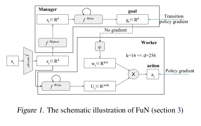
A high-level explanation of the model is as follows:
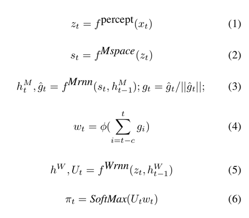
The Manager computes a latent state representation [math]\displaystyle{ s_t }[/math] and outputs a goal vector [math]\displaystyle{ g_t }[/math] . The Worker outputs actions based on the environment observation, its own state, and the Manager’s goal. A perceptual module computes intermediate representation, [math]\displaystyle{ z_t }[/math] of the environment observation [math]\displaystyle{ x_t }[/math], and is shared as input by both Manager and Worker. The Manager’s goals [math]\displaystyle{ g_t }[/math] are trained using an approximate transition policy gradient. The Worker is then trained via intrinsic reward which stimulates it to output actions that will achieve the goals set by the Manager.
Manager and Worker are recurrent networks ([math]\displaystyle{ {h^M} }[/math] and [math]\displaystyle{ {h^W} }[/math] being their internal states). [math]\displaystyle{ \phi }[/math] is a linear transform that maps a goal [math]\displaystyle{ g_t }[/math] into an embedding vector [math]\displaystyle{ w_t \in {R^k} }[/math] , which is then combined with matrix [math]\displaystyle{ U_t }[/math] (Worker's output) via a matrix-vector product to produce policy [math]\displaystyle{ \pi }[/math] – vector of probabilities over primitive actions. The projection [math]\displaystyle{ \phi }[/math] is linear, with no biases, and is learnt with gradients coming from the Worker’s actions.Since [math]\displaystyle{ \phi }[/math] has no biases it can never produce a constant non-zero vector – which is the only way the setup could ignore the Manager’s input. This makes sure that the goal output by the Manager always influences the final policy. In summary, my understanding of the model of goal embedding is: (i) Looking at this model wherein the state is inndependent of, the worker defines a set of partitions of the goal sphere via the embedding function; so each dimension now responds positively to one half of the sphere and negatively to the other half. (ii) Conditioned on the state, the worker then describes each action as a weighted sum of those partitions. Hence, given the state, the worker defines regions of the goal sphere where each action is more likely to be taken.
Learning
The learning considers a standard reinforcement learning setup where the goal of the agent is to maximize the discounted return [math]\displaystyle{ R_t = \sum_{k=0}^{∞} \gamma^k r_{t+k+1} }[/math]; where [math]\displaystyle{ \gamma \in [0,1]; r_t }[/math] is the reward from environment for action at timestep, [math]\displaystyle{ t }[/math]. The agent's behavior is defined by its action-selection policy, [math]\displaystyle{ \pi }[/math].
Since FuN is fully differentiable, the authors could have trained it end-to-end using a policy gradient algorithm operating on the actions taken by the Worker such the outputs [math]\displaystyle{ g }[/math] of the Manager would be trained by gradients coming from the Worker. This, however, would deprive Manager’s goals [math]\displaystyle{ g }[/math] of any semantic meaning, making them just internal latent variables of the model. So instead, Manager is independently trained to predict advantageous directions (transitions) in state space and to intrinsically reward the Worker to follow these directions.
Update rule for manager:
[math]\displaystyle{ \nabla g_t = A_t^M \nabla_\theta d_{cos}(s_{t+c} - s_t, g_t(\theta)) }[/math]
In above equation, [math]\displaystyle{ d_{cos}(\alpha, \beta) = \alpha^T \beta/(|\alpha||\beta|) }[/math] is the cosine similarity between two vectors and [math]\displaystyle{ A_t^M = R_t - V_t^M(x_t,\theta) }[/math] is the Manager’s advantage function, computed using a value function estimate [math]\displaystyle{ V_t^M(x_t,\theta) }[/math] from the internal critic. Here c is an event horizon for the Manager to optimize its direction on. It must be treated as a hyperparameter of the model. It controls the temporal resolution of the Manager. Notice that the last c goals of manager are also first pooled by summation and then embedded into a vector. That makes the conditioning from the manager vary smoothly.
The intrinsic reward that encourages the Worker to follow the goals are defined as:
[math]\displaystyle{ R_t^I = 1/c \sum_{i=1}^c d_{cos}(s_t - s_{t-i}, g_{t-i}) }[/math]
Directions ($s_t - s_{t-i}$)is used because it is more feasible for the Worker to be able to reliably cause directional shifts in the latent state than it is to assume that the Worker can take us to (potentially) arbitrary new absolute locations.
Compared to FRL[3], which advocated concealing the reward from the environment from lower levels of the hierarchy, the Worker in FuN network is trained using an advantage actor-critic[5] to maximise a weighted sum [math]\displaystyle{ R_t + α R_t^I }[/math] , where [math]\displaystyle{ α }[/math] is a hyper-parameter that regulates the influence of the intrinsic reward:
[math]\displaystyle{ \nabla {\pi}_t = A_t^D \nabla_\theta log \pi (a_t|x_t;\theta) }[/math]
The Advantage function [math]\displaystyle{ A_t^D = (R_t + \alpha R_t^I - V_t^D(x_t;\theta)) }[/math] is calculated using an internal critic, which estimates the value functions for both rewards.
The authors also make note of the fact that the Worker and Manager can have different discount factors $\gamma$ for computing return. This allows the Worker to focus on more immediate rewards while the Manager can make decisions over a longer time horizon.
Transition Policy Gradient
The update rule for the Manager given above is a novel form of policy gradient with respect to a model of the Worker’s behavior. The Worker can follow a complex trajectory but it is not necessarily required to learn from these samples. If the trajectories can be predicted, by modeling the transitions, then the policy gradient of the predicted transition can be followed instead of the Worker's actual path. FuN assumes a particular form for the transition model: that the direction in state-space, [math]\displaystyle{ s_{t+c} − s_t }[/math], follows a von Mises-Fisher distribution (it is a probability distribution on the (p-1)-dimensional sphere in Rp, for more information [15]).
Architecture
The perceptual module [math]\displaystyle{ f^{percept} }[/math] is a convolutional network (CNN) followed by a fully connected layer. Each convolutional and fully-connected layer is followed by a rectifier non-linearity. [math]\displaystyle{ f^{Mspace} }[/math], which is another fully connected layer followed by a rectifier non-linearity, is used to compute the state space, which the Manager uses to formulate goals. The Worker’s recurrent network [math]\displaystyle{ f^{Wrnn} }[/math] is a standard LSTM[6].
The Manager uses a novel architecture called a dilated LSTM (dLSTM), which operates at lower temporal resolution than the data stream. It is similar to dilated convolutional networks[7] and clockwork RNN. For a dilation radius r, the network is composed of r separate groups of sub-states or ‘cores’, denoted by [math]\displaystyle{ h = \{\hat{h}^i\}_{i=1}^r }[/math]. At time [math]\displaystyle{ t }[/math], the network is governed by the following equations: [math]\displaystyle{ \hat{h}_t^{t\%r},g_t = LSTM(s_t, \hat{h}_{t-1}^{t\%r};\theta^{LSTM}) }[/math] where % denotes the modulo operation and allows us to indicate which group of cores is currently being updated. At each time step, only the corresponding part of the state is updated and the output is pooled across the previous c outputs. This allows the r groups of cores inside the dLSTM to preserve the memories for long periods, yet the dLSTM as a whole is still able to process and learn from every input experience and is also able to update its output at every step.
Experiments
The baseline the authors are using is a recurrent LSTM[6] network on top of a representation learned by a CNN. The A3C method[5][16] is used for all reinforcement learning experiments. Backpropagation through time (BPTT)[8] is run after K forward passes of a network or if a terminal signal is received. For each method, 100 experiments were run. A training epoch is defined as one million observations. The authors seemed to have ignored Deep Q Learning while comparing the performance results. Speedy Q-learning [14], a new variant of Q-learning algorithm, deals with the problem of slow rate of convergence ( when discount factor [math]\displaystyle{ \gamma }[/math] is close to 1) and achieves a slightly better rate of convergence than other model-based methods. Perhaps, comparisons with these methods could truly assess the power improvements of FeUdal Networks.
Montezuma’s Revenge
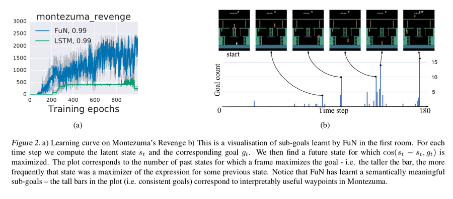
Montezuma’s revenge is a prime example of an environment with sparse rewards. FuN starts learning much earlier and achieves much higher scores. It takes > 300 epochs for LSTM to reach the score 400, which corresponds to solving the first room (take the key, open a door). FuN solves the first room in less than 200 epochs and immediately moves on to explore further, eventually visiting several other rooms and scoring up to 2600 points.
ATARI
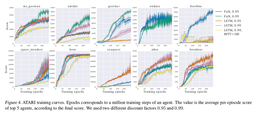
The experiment was run on a diverse set of ATARI games, some of which involve long-term credit assignment and some which are more reactive. Enduro stands out as all the LSTM agents completely fail at it. Frostbite is a hard game that requires both long-term credit assignment and good exploration. The best-performing frostbite agent is FuN with 0.95 Manager discount, which outperforms the rest by a factor of 7. The other results can be seen in the figure.
Comparing the option-critic architecture
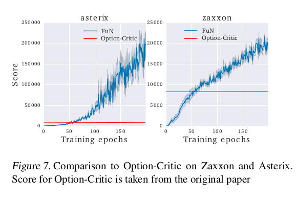
FuN network was run on the same games as Option-Critic (Asterix, Ms. Pacman, Seaquest, and Zaxxon) and after 200 epochs it achieves a similar score on Seaquest, doubles it on Ms. Pacman, more than triples it on Zaxxon and gets more than 20x improvement on Asterix.
Memory in Labyrinth
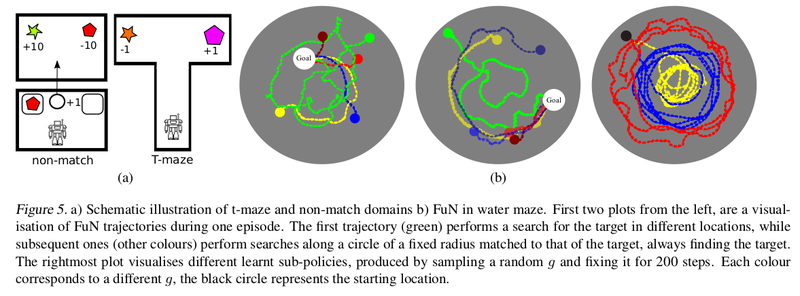
DeepMind Lab (Beattie et al., 2016) is a first-person 3D game platform extended from OpenArena. The games on which the experiments were run on include a Water maze, T-maze, and Non-match (which is a visual memorization task). FuN consistently outperforms the LSTM baseline – it learns faster and also reaches a higher final reward. Interestingly, the LSTM agent doesn’t appear to use its memory for water maze task at all, always circling the maze at the roughly the same radius.
Ablative Analysis
Empirical evaluation of the main contributions of this paper:
Transition policy gradient
Experiments were run on modified FuN networks in which: 1) the Managers output g is trained with gradients coming directly from the Worker and no intrinsic reward is used, 2) g is learned using a standard policy gradient approach with the Manager emitting the mean of a Gaussian distribution from which goals are sampled, 3) a variant of FuN in which g specifies absolute, rather than relative/directional, goals and 4) a purely feudal version of FuN – in which the Worker is trained from the intrinsic reward alone. The experiments (Figure 8) reveal that, although alternatives do work to some degree their performance is significantly inferior.
Temporal resolution ablations
To test the effectiveness of the dilation LSTM, FuN was compared with two baselines 1) the Manager uses a vanilla LSTM with no dilation; 2) FuN with Manager’s prediction horizon c = 1. The non-dilated LSTM fails catastrophically, most likely overwhelmed by the recurrent gradient. Reducing the horizon c to 1 did hurt the performance, although not that much, which means that even at high temporal resolution Manager captures certain properties of the underlying MDP.
Intrinsic motivation weight
Evaluates the effect of weight [math]\displaystyle{ α }[/math] which regulates the relative weight of intrinsic reward. Figure below shows scatter plots of agents final score vs α hyper-parameter where there is a clear improvement in score for high [math]\displaystyle{ \alpha }[/math] in some games.
Dilate LSTM agent baseline
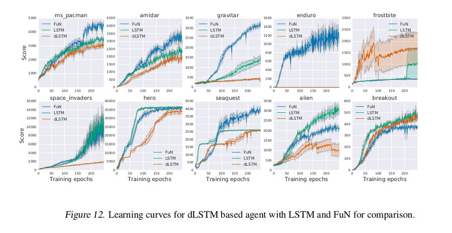
For this experiment, just the dLSTM is used in an agent on top of a CNN, without the rest of FuN structures. Figure below plots the learning curves for FuN, LSTM, and dLSTM agents. dLSTM generally underperforms both LSTM and FuN.
ATARI action repeat transfer
This experiment is to demonstrate the advantage of FeUdal Network, i.e. separating policy and primitive operations. It also implies that the transition policy can be transferred between agents with a different embodiment, for example, across agents with different action repeat on ATARI. The figure below shows the corresponding learning curves. The transferred FuN agent (green curve) significantly outperforms every other method.
Conclusion
FuN is fully differentiable neural network with two levels of hierarchies, currently holds state-of-the-art score in the Atari game, Montezuma's revenge among HRL methods. It is a novel approach to hierarchical reinforcement learning which separates the goal setting behavior from the generation of action primitives. Benefits of this architecture includes better long-term credit assignment, longer memory, emergence of sub-policies as manager learns to select latent goals that maximise extrinsic reward which have been emperically shown in the paper.
Deeper hierarchies by setting goals at multiple time scales is an avenue for further research. The modular structure looks promising for transfer and multitask learning as well.
An implementation of this paper can be found on Github.
As an additional read, as per this report, they have incorporated natural language instructions in the hierarchical RL model to beat the state of the art ATARI systems.
References
- Bacon, Pierre-Luc, Precup, Doina, and Harb, Jean. The option-critic architecture. In AAAI, 2017.
- Bellemare, Marc, Srinivasan, Sriram, Ostrovski, Georg, Schaul, Tom, Saxton, David, and Munos, Remi. Unifying count-based exploration and intrinsic motivation.In NIPS, 2016a.
- Dayan, Peter and Hinton, Geoffrey E. Feudal reinforcement learning. In NIPS. Morgan Kaufmann Publishers,1993.
- Sutton, Richard S, Precup, Doina, and Singh, Satinder. Between mdps and semi-mdps: A framework for temporal abstraction in reinforcement learning. Artificial intelligence, 1999.
- Mnih, Volodymyr, Badia, Adria Puigdomenech, Mirza,Mehdi, Graves, Alex, Lillicrap, Timothy P, Harley, Tim,Silver, David, and Kavukcuoglu, Koray. Asynchronousmethods for deep reinforcement learning. ICML, 2016.
- Hochreiter, Sepp and Schmidhuber, Jürgen. Long short-term memory. Neural computation, 1997.
- Yu, Fisher and Koltun, Vladlen. Multi-scale context aggregation by dilated convolutions. ICLR, 2016.
- Mozer, Michael C. A focused back-propagation algorithm for temporal pattern recognition. Complex systems, 1989.
- Jaderberg, Max, Mnih, Volodymyr, Czarnecki, Wojciech Marian, Schaul, Tom, Leibo, Joel Z, Silver,David, and Kavukcuoglu, Koray. Reinforcement learning with unsupervised auxiliary tasks. arXiv preprint arXiv:1611.05397, 2016.
- A. S. Vezhnevets, S. Osindero, T. Schaul, N. Heess, M. Jaderberg, D. Silver, and K. Kavukcuoglu. Feudal networks for hierarchical reinforcement learning. arXiv preprint arXiv:1703.01161, 2017.
- https://www.quora.com/What-is-hierachical-reinforcement-learning
- Tutorial for Hierarchial Reinforcement Learning: https://www.youtube.com/watch?v=K5MlmO0UJtI
- Videos of FUN agent playing various Atari games can be found in supplementary file accessed through: http://proceedings.mlr.press/v70/vezhnevets17a.html
- Gheshlaghi Azar, Mohammad; Munos, Remi; Ghavamzadeh, Mohammad; Kappen, Hilbert J. (2011). "Speedy Q-Learning". Advances in Neural Information Processing Systems. 24: 2411–2419.
- https://en.wikipedia.org/wiki/Von_Mises%E2%80%93Fisher_distribution
- https://medium.com/emergent-future/simple-reinforcement-learning-with-tensorflow-part-8-asynchronous-actor-critic-agents-a3c-c88f72a5e9f2
