kernel Dimension Reduction in Regression: Difference between revisions
No edit summary |
m (Conversion script moved page Kernel Dimension Reduction in Regression to kernel Dimension Reduction in Regression: Converting page titles to lowercase) |
| (One intermediate revision by one other user not shown) | |
(No difference)
| |
Latest revision as of 09:46, 30 August 2017
The problem of Sufficient Dimension Reduction(SDR) for regression is to find a subspace such that covariates are conditionally independent given the subspace. In classical SDR regression methods, marginal distribution of explanatory variables are needed to calculate the independency measurement. This paper proposes that conditional independence can be characterized in terms of conditional covariance operators on Reproducing Kernel Hilbert Spaces(RKHS). This is the first few papers on independency measurement in RKHS(Other recent methods are the RHIC and dCor).
Sufficient Dimension Reduction(SDR)
The problem of SDR for regression is that of finding a subspace S such that the projection of the covariate vector X onto S captures the statistical dependency of the response Y on X[ref]. That is: [math]\displaystyle{ Y\perp X | \Pi_S X }[/math] Where [math]\displaystyle{ \Pi_S X }[/math] denotes the orthogonal projection of X on to S. performing a regression of X on Y generally requires making assumptions with respect to the probability distribution of X which can be hard to justify[ref]. Most of the previous regression methods assume linearity between projected X and Y. This assumption only stand when the distribution of X is elliptic.
Cross-covariance operator
Cross-covariance operator is first propose by (Baker,1973). It can be used to measure the relations between probability measures on two RKHSs. Define two RKHSs [math]\displaystyle{ H_1 }[/math] and [math]\displaystyle{ H_2 }[/math] with inner product [math]\displaystyle{ \lt .,.\gt _1 }[/math], [math]\displaystyle{ \lt .,.\gt _2 }[/math]. A probability measure [math]\displaystyle{ \mu_i }[/math] on [math]\displaystyle{ H_i,i=1,2 }[/math] that satisfies
[math]\displaystyle{ \int_{H_i}||x||_i^2d\mu_i(x)\lt \infty }[/math]
defines an operator [math]\displaystyle{ R_i }[/math] in [math]\displaystyle{ H_i }[/math] by
[math]\displaystyle{ \lt R_iu,v\gt =\int_{H_i}\lt x-m_i,u\gt _i\lt x-m_i,v\gt _id\mu_i(x) }[/math]
[math]\displaystyle{ R_i }[/math] is called covariance operator, if u and v are in different RKHS, then [math]\displaystyle{ R_i }[/math] is called cross-covariance operator.
Kernel Dimension Reduction for Regression
This paper calculate conditional independency measurements by using conditional covariance operators in RKHS. No strong assumptions are needed on [math]\displaystyle{ P_{\Pi_S}(Y|\Pi_S X) }[/math] or P(X). Let [math]\displaystyle{ (H_x,k_x) }[/math] and [math]\displaystyle{ (H_y,k_y) }[/math] be RKHS's of functions on X and Y. The cross-covariance operator of (X,Y) from [math]\displaystyle{ H_x }[/math] to [math]\displaystyle{ H_y }[/math] can be defined as
[math]\displaystyle{ \lt \sum{_{YX}}f , g\gt _{H_y} = E_{XY}[(f(X)-E_X{[f(X)]})(g(Y)-E_Y{[g(Y)]})] }[/math]
It holds for all f in Hx and g in Hy. [math]\displaystyle{ \sum{_{XX}},\sum{_{YY}} }[/math]can be defined likewise. A important theorem is that
[math]\displaystyle{ \sum{_{YY|X}}=\sum{_{YY}}-\sum{_{YX}}\sum{_{XX}}^{-1}\sum{_{XY}} }[/math]
Now assume a unknown projection matrix B that projects n dimensional X into a d dimensional subspace U by [math]\displaystyle{ U=B^TX }[/math] The SDR criterion can be rewrite to [math]\displaystyle{ B = \arg \min_B \sum{_{YY|U}} }[/math] It makes sense that when U captures most of the relationship between X and Y, given U, Y is much determined, so the conditional covariance operator should be small. It can be proved that when [math]\displaystyle{ \sum{_{YY|U}}=\sum{_{YY|X}} }[/math], X and Y are conditionally independent given U, and [math]\displaystyle{ \sum{_{YY|U}}\gt \sum{_{YY|X}} }[/math].
Define [math]\displaystyle{ \tilde{k_1}^{(i)} \in H_1 }[/math] by [math]\displaystyle{ \tilde{k_i}^{(i)}=K_1(\cdot,Y_i)-\frac{1}{n}\sum_{j=1}^{n}K_1(\cdot,Y_j) }[/math]. [math]\displaystyle{ \tilde{k_1}^{(i)} \in H_2 }[/math] similarly using [math]\displaystyle{ U }[/math]. Notice The relationship between space U and space X is [math]\displaystyle{ K_2(B^Tx,B^T\tilde{x})=K_x{x,\tilde{x}} }[/math]. Optimize B can be done by optimize U and derive B from U from there relationship.
replace the expectation with the empirical average,
[math]\displaystyle{ \lt f, \sum{_{YU}}g\gt _{H_1} \approx \frac{1}{n}\sum_{i=1}^n \lt \tilde{k_1}^{(i)},f\gt \lt \tilde{k_2}^{(i)},g\gt . }[/math]
Let [math]\displaystyle{ \hat{K_Y} }[/math] be the centralized Gram matrix,
[math]\displaystyle{ \hat{K_Y}=(I_n-\frac{1}{n}1_n1_n^T)G_Y(I_n-\frac{1}{n}1_n1_n^T) }[/math] in which [math]\displaystyle{ 1_n=(1,1,...,1)^T }[/math]
Then it's easy to see that
[math]\displaystyle{ \lt \tilde{k_1}^{(i)},\tilde{k_1}^{(j)}\gt =\hat{K_Y} }[/math]
[math]\displaystyle{ \lt \tilde{k_2}^{(i)},\tilde{k_2}^{(j)}\gt =\hat{K_U} }[/math]
if we approximate f and g as
[math]\displaystyle{ f=\sum_{l=1}{n}a_l\tilde{k_1}^{(l)} }[/math]
[math]\displaystyle{ g=\sum_{m=1}{n}b_m\tilde{k_2}^{(m)} }[/math]
Then the covariance is approximated by
[math]\displaystyle{ \lt f,\sum{_{YU}}g\gt _{H_1}=\sum_{l=1}{n}\sum_{m=1}{n}a_lb_m(\hat{K}_Y\hat{K}_U)_{lm} }[/math]
That is [math]\displaystyle{ \sum{_{YU}}=\hat{K}_Y\hat{K}_U }[/math].
[math]\displaystyle{ \sum{_{YY}} }[/math] and [math]\displaystyle{ \sum{_{UU}} }[/math] can be estimated similarly except a regulation need to be added to make sure the optimization gives a useful result[ref]. The empirical conditional covariance matrix is then estimate by
[math]\displaystyle{ \sum{_{YY|U}}:=\hat{\sum}{_{YY}}-\hat{\sum}{_{YU}}(\hat{\sum}{_{UU}}+\varepsilon_nI)^{-1}\hat{\sum}{_{UY}} }[/math]
Optimization
Minimize this conditional covariance matrix on U, then B can be derived. The "size" of this conditional covariance matrix can be evaluated by it's trace,
Test Results
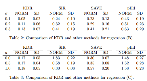
The results are evaluated by [math]\displaystyle{ B_0B_0^T-\hat{B}\hat{B}^T }[/math]_F where [math]\displaystyle{ B_0 }[/math] and [math]\displaystyle{ \hat{B} }[/math] are the true subspace and estimated subspace respectively. Gaussian RBF kernel [math]\displaystyle{ exp(-||z_1-z_2||^2/c) }[/math] is used. [math]\displaystyle{ c=0.5 }[/math]. [math]\displaystyle{ \varepsilon=0.1 }[/math]. E follows a standard Gaussian Distribution [math]\displaystyle{ N(0,1) }[/math]
Three regression functions:
(A) [math]\displaystyle{ Y=\frac{X_1}{0.5+(X_2+1.5)^2}+(1+X_2)^2\lt +\sigma E }[/math]
(B) [math]\displaystyle{ Y=sin^2(\pi X_2+1)+\sigma E }[/math]
(C) [math]\displaystyle{ Y=\frac{1}{2}(X_1-a)^2E }[/math]
The next three tables are the regression results in comparison with three other SDR algorithms
Discussion
The author is the fist few people who proposed to use RKHS for independency measurement. The main improvement to previous methods is that the independency is measured in RKHS, it implicitly tested all possible functions between Y and X. No linearity or distribution assumption is needed.
References
[1] Fukumizu, Kenji, Francis R. Bach, and Michael I. Jordan. "Kernel dimension reduction in regression." The Annals of Statistics 37.4 (2009): 1871-1905.
[2] Fukumizu, Kenji, Francis R. Bach, and Michael I. Jordan. "Dimensionality reduction for supervised learning with reproducing kernel Hilbert spaces." The Journal of Machine Learning Research 5 (2004): 73-99.
[3] Bach, Francis R., and Michael I. Jordan. "Kernel independent component analysis." The Journal of Machine Learning Research 3 (2003): 1-48.
[4] Baker, Charles R. "Joint measures and cross-covariance operators." Transactions of the American Mathematical Society 186 (1973): 273-289.

