The Stochastic Pendulum with white noise

This script is a tutorial script for stochastic integration and visualization using white noise.

The governing ODEs of the damped pendulum are
This section is all the book keeping for initialization
The parameters for the white noise
Initial conditions
Set up arrays for storage and store initial state
The main work horse loops. The double loop can be used view to intermediate results
Now that we have the data we can make a variety of pictures

The governing ODEs of the damped pendulum are

$\theta' = v$

$v' = -\frac{g}{l} \sin{\theta} - damping*v$

$g$ is taken to vary as $g_0*(1+perturbation)$ where the perturbation is white noise. This script uses the Euler-Maruyama method for solving the DE which uses Ito calculus. To use Ito calculus we write the system as:

$d\theta = v dt$ (no stochastic component)

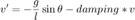
$v'=[-\frac{g}{l} \sin{\theta} - damping*v]*dt - noiseamp*(g0/L)*sin(theta)*dW$

Then discretize using the usual stochastic calculus way. This is opposed to Stratonavich calculus, however we can convert between the two using the Ito-Stratonovich drift correction formula:

$dV = f(V, \theta)dt + g(V, \theta)dW$ (Ito)

$dV = f_bar(V, \theta)dt + g(V, \theta)dW$ (Stratonavich)

where $f_bar(V, \theta) = f(V, \theta) - 1/2 g(V, \theta)g'(V, \theta)$ . In this particular case $g(V)$ does not depend on $V$ and so $f_bar(V) = f(V)$ .

This section is all the book keeping for initialization

Initialize the random number generator and seed it.

rng('shuffle');

Specify the global parameters for the pendulum.

length=1;
g0=9.81;
damp=1e-1;

Specify the time step and stochastic parameters.

numsteps=10; % Sets how many time steps between saves.
numouts=100; % Sets the number of outputs.
dt=1e-3; % Sets the time step.
dtrt=sqrt(dt); % For the white noise.

Stochastic methods are low order so small time steps are required. Sets the number of ensemble members.

numens=1000;

The parameters for the white noise

Set the standard deviation of the noise.

mysig=0.35;

Initial conditions

% theta=2*pi*rand(numens,1); %initially assume random angles
theta=(1-1e-4)*pi*ones(numens,1); % start near the unstable state
% theta=1e-4*pi*ones(numens,1); % start near the stable state
v=zeros(numens,1); % Initially assume zero velocity.
t=0;

Set up arrays for storage and store initial state

thetas=zeros(numouts+1,numens);
vs=zeros(numouts+1,numens);
ts=zeros(numouts+1,1);
thetas(1,:)=theta;
vs(1,:)=v;
ts(1)=t;

The main work horse loops. The double loop can be used view to intermediate results

for ii=1:numouts
    for jj=1:numsteps

Generate a new bunch of random numbers.

        nowrand=randn(numens,1)*mysig;

Define the rhs for the DE.

        rhth=v;

The deterministic part.

        rhv=-(g0/length).*sin(theta)-damp*v;

The stochastic part.

        rhvstoch = (-g0/length).*sin(theta);
        theta=theta+dt*rhth+dtrt*nowrand.*rhvstoch;
        v=v+dt*rhv;
        t=t+dt;

    end
    thetas(ii+1,:)=theta;
    vs(ii+1,:)=v;
    ts(ii+1)=t;
end

Now that we have the data we can make a variety of pictures

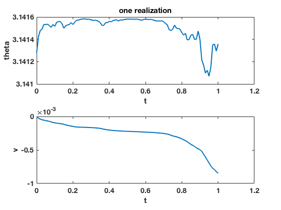
figure(1)
clf
set(gcf,'DefaultLineLineWidth',2,'DefaultTextFontSize',14,...
    'DefaultTextFontWeight','bold','DefaultAxesFontSize',14,...
    'DefaultAxesFontWeight','bold');
subplot(2,1,1)
plot(ts,thetas(:,1))
xlabel('t')
ylabel('theta')
title('one realization')
subplot(2,1,2)
plot(ts,vs(:,1))
xlabel('t')
ylabel('v')

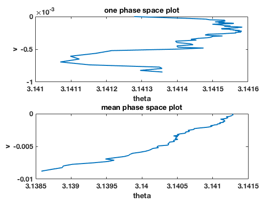
figure(2)
clf
set(gcf,'DefaultLineLineWidth',2,'DefaultTextFontSize',14,...
    'DefaultTextFontWeight','bold','DefaultAxesFontSize',14,...
    'DefaultAxesFontWeight','bold');
subplot(2,1,1)
plot(thetas(:,1),vs(:,1))
ylabel('v')
xlabel('theta')
title('one phase space plot')
subplot(2,1,2)
plot(mean(thetas,2),mean(vs,2))
ylabel('v')
xlabel('theta')
title('mean phase space plot')

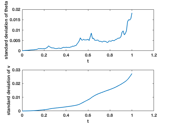
figure(3)
clf
set(gcf,'DefaultLineLineWidth',2,'DefaultTextFontSize',14,...
    'DefaultTextFontWeight','bold','DefaultAxesFontSize',14,...
    'DefaultAxesFontWeight','bold');
subplot(2,1,1)
plot(ts,std(thetas,[],2))
ylabel('standard deviation of theta')
xlabel('t')
subplot(2,1,2)
plot(ts,std(vs,[],2))
ylabel('standard deviation of v')
xlabel('t')

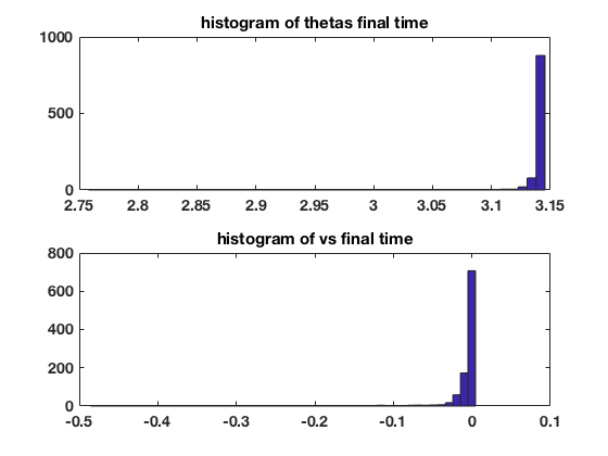
figure(4)
clf
set(gcf,'DefaultLineLineWidth',2,'DefaultTextFontSize',14,...
    'DefaultTextFontWeight','bold','DefaultAxesFontSize',14,...
    'DefaultAxesFontWeight','bold');
subplot(2,1,1)
mnth=min(thetas(end,:));
mxth=max(thetas(end,:));
bins=linspace(mnth,mxth,floor(numens/20)+1);
hist(thetas(end,:),bins)
title('histogram of thetas final time')
subplot(2,1,2)
mnv=min(vs(end,:));
mxv=max(vs(end,:));
bins=linspace(mnv,mxv,floor(numens/20)+1);
hist(vs(end,:),bins)
title('histogram of vs final time')