Ito vs Stratonovich
This script is an implementation of a really simple stochastic ODE to show the difference between Ito and Stratonovich calculus. Please note that this script defines functions at the end, which is only supported by MATLAB 2016b or later.
Contents
the SDE has the form:

Ito calculus is handled by the standard Euler Maruyama scheme:


Stratonovich calculus is handled by the Euler Heun scheme:
![$$ x^n+1=x^n + f(x^n,t^n) \Delta t + \Delta W*[g(x^n,t^n)+g(\bar{x},t^n)]/2. $$](stoch_ito_stratonovich_eq04649210088799611819.png)
Note that for additive noise g is a constant so the two are the same.
The Stratonovich interpretation effectively adds a drift.
clear all, close all
% Initialize the random number generator and seed it.
rng('shuffle');
Specify the global parameters.
mysig=1;
myper=3e-2;
Specify the time step and stochastic parameters.
numsteps=10;
numouts=100;
dt=1e-5;
dtrt=sqrt(dt);
dtb=dt*numsteps;
dtbrt=sqrt(dtb);
numens=4000;
Set up arrays for storage and store initial state.
t=0;
xs=zeros(numouts+1,numens);
xi=zeros(numouts+1,numens);
x0=zeros(1,numens);
xs(1,:)=x0;
xi(1,:)=x0;
xd=x0(1);x=x0;x2=x0;
ts(1)=t;
cntr=0;
xs(1,:)=x;
xds(1)=xd;
ts(1)=t;
Primary loop
for ii=1:numouts
for jj=1:numsteps
        cntr=cntr+1;
        noisenow=randn(1,numens);
Euler Maruyama.
x=x+dt*sin(2*pi*t/myper)+dtrt*mysig*noisenow.*atan(x)*(2/pi);
Euler-Heun.
        x2bar=x2+mysig*noisenow.*atan(x)*(2/pi);
        x2=x2+dt*sin(2*pi*t/myper)+0.5*dtrt*mysig*noisenow.*(atan(x2bar)*(2/pi)+atan(x2)*(2/pi));
t=t+dt;
end
Storage
    xs(ii+1,:)=x2;
    xi(ii+1,:)=x;
    ts(ii+1)=t;
end
Plotting
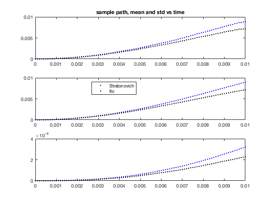
Plot one path, mean and standard deviation.
figure(1)
clf
subplot(3,1,1)
plot(ts,xs(:,1),'b.',ts,xi(:,1),'k.')
title('sample path, mean and std vs time')
subplot(3,1,2)
plot(ts,mean(xs,2),'b.',ts,mean(xi,2),'k.')
legend('Stratonovich','Ito','Location','best')
subplot(3,1,3)
plot(ts,std(xs,[],2),'b.',ts,std(xi,[],2),'k.')
Derivative-free Milstein Method Ito
function x_next =  dfmil_ito(x_n,f_n,g_n,h)
    x_bar = x_n + feval(f_n,x_n)*h + feval(g_n,x_n)*sqrt(h);
    x_next = x_n + feval(f_n,x_n)*h + feval(g_n,x_n)*sqrt(h)*randn + 0.5*h^(-0.5)*(feval(g_n,x_bar)-feval(g_n,x_n))*(h*randn^2-h);
end
Derivative-free Milstein Method Stratonovich
function x_next =  dfmil_strat(x_n,f_n,g_n,h)
    x_bar = x_n + feval(f_n,x_n)*h + feval(g_n,x_n)*sqrt(h);
    x_next = x_n + feval(f_n,x_n)*h + feval(g_n,x_n)*sqrt(h)*randn + 0.5*h^(-0.5)*(feval(g_n,x_bar)-feval(g_n,x_n))*(h*randn^2);
end