Gillespie's Algorithm (SSA)

This script implements Gillespie's Algorithm taking advantage of Matlab's vector operations. The for loops have been kept at a minimum. Gillespie's Algorithm is considered an exact stochastic simulation, however the downside is that it is much more computationally expensive than other approximate methods. This is why so much effort was put into vectorizing the script. In this model we have four species of partivles and eight possible reations that can occur. The method works by using a logarithmic distribution to find the time until the next reaction occurs, and then randomly picks from the reactions which occurs and then updates the species. For more information on the method please see (Gillespie, 1977). The parameters here are based off of Morshed et al., 2017 in BioSystems.

Contents

close all;clear;
rng ('shuffle');

Parameters

We have four species, eight reactions, an ensemble of 10000 and will let it run for 100 reactions.

n_species = 4;
n_paths = 8;
n_react = 1e2;
n_ens = 100;

Constants

epsilon = 0.05;
stiff = 1000;
alpha1 = 1.26;
alpha2 = 1.26;
beta = 4;
gamma = 4;
ii1 = 0;
ii2 = 0;
c(1)=alpha1*23;
c(2)=0.23;
c(3)=0.23;
c(4)=0.23;
c(5)=alpha2*23;
c(6)=0.23;
c(7)=0.23;
c(8)=0.23;

Reaction Matrix

This defines the results of the various reactions on the species.

react_result = [0  0   1   0;
                0  0   -1  0;
                1  0   0   0;
                -1 0   0   0;
                0  0   0   1;
                0  0   0   -1;
                0  1   0   0;
                0  -1  0   0];

Initial numbers set to zero

X0 = [76;75;60;60];
n_mol = repmat(X0,1,n_ens);
prop = zeros(n_paths,n_ens);
react_result=repmat(react_result,1,1,n_ens);
ti=zeros(1,n_ens);
tn=ti;
cntr=0;
for ii=1:n_react

Propensities

The propensity of each reaction.

    prop(1,:) = (stiff*c(1)*(1+ii2)^beta)./(1+ii2+0.01*n_mol(2,:)).^beta;
    prop(2,:) = stiff*c(2)*n_mol(3,:);
    prop(3,:) = c(3)*n_mol(3,:);
    prop(4,:) = c(4)*n_mol(1,:);
    prop(5,:) = stiff*(c(5)./(1+((0.01*n_mol(1,:))./(1+ii1)).^gamma));
    prop(6,:) = stiff*c(6)*n_mol(4,:);
    prop(7,:) = c(7)*n_mol(4,:);
    prop(8,:) = c(8)*n_mol(2,:);

Time to next reaction

    deltat=-log(rand(1,n_ens))./sum(prop);
    tn = tn + deltat;

See valid reactions

The greater than returns a logical matrix which I then element-wise multiply to keep the matrix the same size.

    valid_ind = prop>0;
    valid_prop = prop.*valid_ind;
    valid_ind_3d = repmat(valid_ind,1,1,n_species);
    valid_ind_3d = reshape(valid_ind_3d,[n_paths n_species n_ens]);
    valid_result = react_result.*valid_ind_3d;

Record the locations of zeros.

    invalid=~logical(valid_prop);

Probability intervals

I take advantage that the default for most operations is to apply them column-wise.

    prop_int = cumsum(valid_prop);
    % Set the invalid paths to NaN to not mess anything up.
    prop_int(invalid)=NaN;

Normalize

Use bsxfun to normalize each row (species) of the propensity intervals by a vector that is the maximum of each column,

    prop_int = bsxfun(@rdivide,prop_int,max(prop_int));

Pick the reaction

Make the random vector with one number for each ensemble member.

    rand_react = rand(1,n_ens);

Find all propensity intervals that are greater than the random number for each ensemble (column).

    react_ind = bsxfun(@gt,prop_int,rand_react);

Find the index of the first entry in each column that is nonzero.

    [~,ind] = max(react_ind~=0,[],1);

Since this gives the respective row index that the first nonzero entry appears we need to multiply by the number of species times the ensemble number to get the position in linear indexing. Had to make this more complicated for the general case. This is the starting index for each of the corresponding rows in linear indexing.

    start_ind = (0:n_ens-1).*n_species.*n_paths + (1 + n_species.*(ind-1));

Since we want the entire 'row' or all the species

    species = 0:n_species-1;

Add replicated versions of the two vectors to endup with all the relavent indices.

    indicies = bsxfun(@plus,repmat(start_ind,n_species,1),repmat(species(:),1,n_ens));

Add the valid result for to each species for the current number of mols.

    n_mol = n_mol+valid_result(indicies);

end

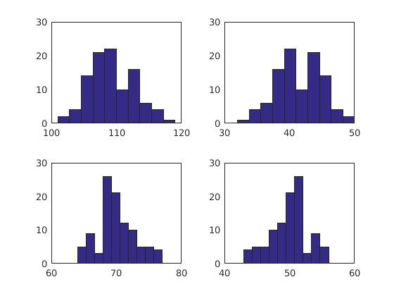
Plot

figure(1)
clf
subplot(2,2,1)
hist(n_mol(1,:))
subplot(2,2,2)
hist(n_mol(2,:))
subplot(2,2,3)
hist(n_mol(3,:))
subplot(2,2,4)
hist(n_mol(4,:))

Published with MATLAB® R2016b