The Stochastic potential well with driving and red noise

This script is a tutorial script for stochastic integration and visualization using red noise realized using the method of Bartosch. The governing ODEs of the system are: x'=v v'=-V'(x)-damping*v+f_deterministic+f_stochastic; where V(x) is the potential of interest. A tilted double well potential is implemented in this code.

Contents

This section is all the book keeping for initialization

Initialize the random number generator and seed it.

rng('shuffle');

Specify the global parameters for the pendulum

L=5;
x0deep=-3;
x0shal=3;
wellslope=2;
dxnum=1e-8;
myV=@(xnow) ((xnow-x0deep).*(xnow-x0shal)).^2+wellslope*xnow;
myVp=@(xnow) (myV(xnow+dxnum)-myV(xnow-dxnum))./(2*dxnum);
damp=8e-1;
myamp=15; myper=2;
myforce=@(t) myamp*sin(2*pi*t/myper);

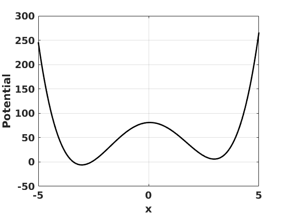
Bi-stable Potential Well

figure(1)
clf
set(gcf,'DefaultLineLineWidth',2,'DefaultTextFontSize',14,...
    'DefaultTextFontWeight','bold','DefaultAxesFontSize',14,...
    'DefaultAxesFontWeight','bold');
wellxs=linspace(-5,5,1001);
plot(wellxs,myV(wellxs),'k-')
grid on
xlabel('x')
ylabel('Potential')

Specify the time step and stochastic parameters

numsteps=10; % Sets how many time steps between saves.
numouts=200; % Sets the number of outputs.
dt=1e-3; % sets the time step.  Stochastic methods are low order so small time steps are required.
numens=100; % Sets the number of ensemble members.

The parameters for the red noise as realized by Bartosch's algorithm

memt=0.2; % Sets the memory of the noise.  Need at least ten time steps in memt.
rho=exp(-dt/memt); rhoc=sqrt(1-rho*rho); % Parameters for Bartosch's method.
%mysig=40; % Set the standard deviation of the noise. This is strong noise
mysig=30; % Set the standard deviation of the noise. This is medium noise
prevrand=zeros(numens,1); % Start g at g0.

Initial conditions

x=x0shal*ones(numens,1); % Start near the shallow well location.
% x=1e-4*pi*ones(numens,1); % Start nearthe stable state.
v=zeros(numens,1); % Initially assume zero velocity.
t=0;

Set up arrays for storage and store initial state

xs=zeros(numouts+1,numens);
vs=zeros(numouts+1,numens);
ts=zeros(numouts+1,1);
xs(1,:)=x;
vs(1,:)=v;
ts(1)=t;

The main work horse loops. The double loop can be used view to intermediate results

for ii=1:numouts
    for jj=1:numsteps

        nowrand=randn(numens,1)*mysig; % Generate a new bunch of random numbers.
        pertnow=(nowrand*rhoc+rho*prevrand);
        prevrand=pertnow; % Use Bartosch's memory to get the right "memory".

Define the rhs for the DE.

        rhth=v;
        rhv=-myVp(x)-damp*v+pertnow+myforce(t)*ones(numens,1);

Step the DE forward. If g had a white noise component this would get trickier to account for the sqrt(dt) in Ito's calculus.

        x=x+dt*rhth;
        v=v+dt*rhv;
        t=t+dt;

    end
    xs(ii+1,:)=x;
    vs(ii+1,:)=v;
    ts(ii+1)=t;
end

Now that we have the data we can make a variety of pictures

figure(2)
clf
set(gcf,'DefaultLineLineWidth',2,'DefaultTextFontSize',14,...
    'DefaultTextFontWeight','bold','DefaultAxesFontSize',14,...
    'DefaultAxesFontWeight','bold');
subplot(2,1,1)
plot(ts,xs(:,1))
xlabel('t')
ylabel('x')
title('one realization')
subplot(2,1,2)
plot(ts,vs(:,1))
xlabel('t')
ylabel('v')

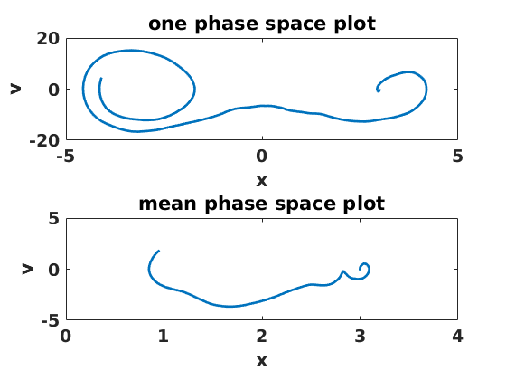
figure(3)
clf
set(gcf,'DefaultLineLineWidth',2,'DefaultTextFontSize',14,...
    'DefaultTextFontWeight','bold','DefaultAxesFontSize',14,...
    'DefaultAxesFontWeight','bold');
subplot(2,1,1)
plot(xs(:,1),vs(:,1))
ylabel('v')
xlabel('x')
title('one phase space plot')
subplot(2,1,2)
plot(mean(xs,2),mean(vs,2))
ylabel('v')
xlabel('x')
title('mean phase space plot')

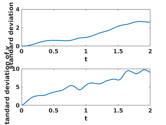
figure(4)
clf
set(gcf,'DefaultLineLineWidth',2,'DefaultTextFontSize',14,...
    'DefaultTextFontWeight','bold','DefaultAxesFontSize',14,...
    'DefaultAxesFontWeight','bold');
subplot(2,1,1)
plot(ts,std(xs,[],2))
ylabel('standard deviation of x')
xlabel('t')
subplot(2,1,2)
plot(ts,std(vs,[],2))
ylabel('standard deviation of v')
xlabel('t')

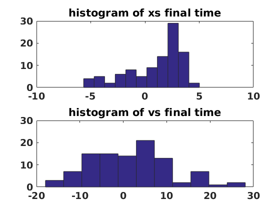
figure(5)
clf
set(gcf,'DefaultLineLineWidth',2,'DefaultTextFontSize',14,...
    'DefaultTextFontWeight','bold','DefaultAxesFontSize',14,...
    'DefaultAxesFontWeight','bold');
subplot(2,1,1)
mnth=min(xs(end,:));
mxth=max(xs(end,:));
bins=linspace(mnth,mxth,floor(numens/10)+1);
hist(xs(end,:),bins)
title('histogram of xs final time')
subplot(2,1,2)
mnv=min(vs(end,:));
mxv=max(vs(end,:));
bins=linspace(mnv,mxv,floor(numens/10)+1);
hist(vs(end,:),bins)
title('histogram of vs final time')

Waiting Time Computation

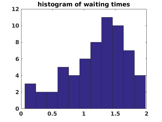
We now compute waiting times. These are a standard part of analysis for many stochastic systems. In this case the waiting times can be used to characterize the phenomenon of stochastic resonance (basically by looking at the histogram of waiting times and seeing if multiples of the period of the deterministic driving are evident). The waiting time is defined as the time it takes to move from one well to the other. That means we can use the unstable equilibrium point between the two wells to calculate the waiting time.

waits=[];

Set how close to the unstable equilibrium is close enough.

myeps=0.1;

Now find the unstable equilibrium point.

xnow=linspace(-1,1,1001);
vv=myV(xnow);
[aa bb]=max(xnow);
xtop=xnow(bb);
for ii=1:numens

    xnow=xs(:,ii);
    crossings=find(abs(xnow-xtop)<myeps);

Find the crossings and make sure the set isn't empty.

    if isempty(crossings)==0

        waitnow=[];
        waitnow(1)=crossings(1);
        dummy=diff(crossings);
        tooshorts=find(dummy<2);

Only keep data if we're not fidgeting around the equilibrium.

        dummy(tooshorts)=[];
        waitnow=[waitnow;dummy];
        waits=[waits;waitnow];

    end

end
waits=waits*dt*numsteps; % Scale.

figure(6)
clf
set(gcf,'DefaultLineLineWidth',2,'DefaultTextFontSize',14,...
    'DefaultTextFontWeight','bold','DefaultAxesFontSize',14,...
    'DefaultAxesFontWeight','bold');
hist(waits,floor(numens/10)+1)
title('histogram of waiting times')

Published with MATLAB® R2016b