2D Spectral Analysis

This script shows you how to perform 2D spectral analysis by looking at the spectrum along the radial direction in wavenumber space. This allows you to reduce a dimension and plot the information in a manner similar to the 1D spectra.

Create the grid
Create the function
Take the FFT2
Compute the radial spectrum
Plots

Create the grid

Nx = 512;
Ny  = 512;
Lx  = 1e2;
Ly  = 1e2;

Grid Spacing.

dx=Lx/Nx;
dy=Ly/Ny;

Create the x and y axis'.

x=dx*(1:Nx)';
y=dy*(1:Ny)';

Create the grid.

[xx,yy]=meshgrid(x,y);

Wavenumber spacing.

dk = 2*pi/Lx;
dl = 2*pi/Ly;

Wavenumber grid.

k = [0:Nx/2 -Nx/2+1:-1]'*dk;
l = [0:Ny/2 -Ny/2+1:-1]'*dl;
[kk,ll]=meshgrid(k,l);
kksh=fftshift(kk);
llsh=fftshift(ll);
kmag=sqrt(kk.^2+ll.^2);
myfilt=exp(-(kmag/3).^2);
kmag=sqrt(kk.^2+ll.^2);
kmagv=kmag(:);

Create the function

rr=sqrt((xx-0.5*Lx).^2+(yy-0.5*Ly).^2);
myf=exp(-(rr/(0.2*Lx)).^2).*sin(2*pi*xx/(0.1*Lx)).*sin(2*pi*yy/(0.05*Ly))+randn(size(xx))*0.0001;

Take the FFT2

We use the 2D FFT fft2. We also use the function "fftshift" to shift the zero-frequency component to the center of the spectrum.

myspec=abs(fft2(myf));
myspecsh=fftshift(myspec);
myspecv=myspec(:);

Compute the radial spectrum

We set a number of bins which are shells around the center.

Nbins=80;
mxk=min(max(k),max(l));
dk=mxk/Nbins;
for ii=1:Nbins

The filter for the shell.

    myfilt=(kmagv<ii*dk&kmagv>(ii-1)*dk);

The mean over the shell.

    myradspec(ii)=sum(myspecv.*myfilt)/sum(myfilt);

end

Plots

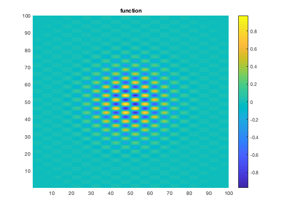
The original function.

figure(1)
clf
pcolor(xx,yy,myf)
shading interp,colorbar
title('function')

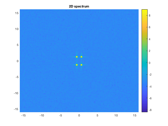
The 2D spectrum.

figure(2)
clf
pcolor(kksh,llsh,log((myspecsh)))
shading interp,colorbar
title('2D spectrum')

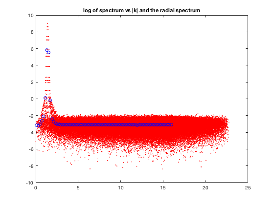
The radial spectrum. In red is the raw vectorized version of the 2D plot. While in blue is the radially averaged version.