Spectral Windowing and Variance Reduction
This script illustrates how to use windowing to get localized signal information and how to reduce the spatial/temporal variance. We will be using some of the simplifications outlined in the intro_spectral1d.m script.
Contents
close all;clear;
Make a grid and wavenumbers
N = 1024;
L = 20;
z = linspace(-1,1,N+1);
z = z(1:end-1);
x = z*L;
dx = x(2)-x(1);
dk = pi/L;
ksvec = 0:N/2-1;
k = ksvec'*dk;
Sample Function
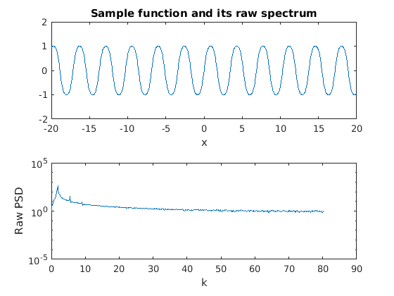
For this example we will use the a more complicated function, the Jacobi Elliptic function. This function has clearly a clearly defined spectrum with peaks at 1.885 and 5.498. We then add a random perturbation to this signal.
[fs,~,~]=ellipj(2*pi*x/2.5,0.75);
f1=fs+0.005*randn(size(x));
fft_f1 = abs(fft(f1));
PSD with no windowing
Without any windowing we can see that the spectrum is extremely problematic. While there are peaks at the correct wavenumbers, there is power at every wavenumber and there are small oscillations at large wavenumbers.
figure(1)
subplot(2,1,1)
plot(x,f1)
xlabel('x')
title('Sample function and its raw spectrum')
subplot(2,1,2)
semilogy(k,fft_f1(1:end/2))
xlabel('k')
ylabel('Raw PSD')
Windowing
These problems can be partially solved by windowing. Windowing is multiplying the original function by a "window" function that is localized You can think of windowing like making a packet from your signal. Here we specify the center point (N/2) and then the windowing function linearly decreases from there.
No2 = N/2;
mywin = [0:No2-1 No2:-1:1]/No2;
f1w = mywin.*f1;
fft_f1w = abs(fft(f1w));
figure(2)
subplot(2,1,1)
plot(x,f1,'b',x,f1w,'r')
title('Sample function, windowed function and their spectra')
subplot(2,1,2)
semilogy(k,fft_f1(1:end/2),'b',k,fft_f1w(1:end/2),'r')
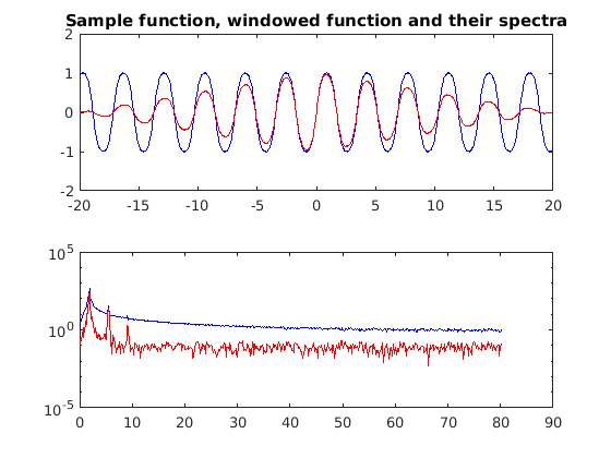
You can see that this has decreased the power at most wavenumbers however we still have problems. The windowed spectrum is more choppy.
Variance Reduction
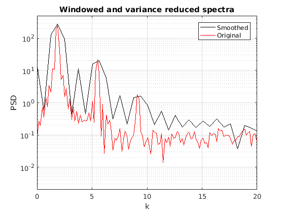
Using abs(fft(f)) gives an estimate of the spectrum with a lot of variance (technically an astonishing 100%). In practice things are rarely that bad, but when a signal is long the variance can be reduced by splitting the signal up, windowing each piece and summing.
No4 = N/4;
mywin = [0:No4/2-1 No4/2:-1:1]/(No4/2);
myspec = zeros(No4,1)';
for ii=0:3
    fnow = mywin.*f1(ii*No4+1:(ii+1)*No4);
    myspec = myspec+abs(fft(fnow));
end
dk4 = 4*pi/L;
k4svec = 0:No4/2-1;
k4 = k4svec'*dk4;
figure(3)
semilogy(k4,myspec(1:end/2),'k',k,fft_f1w(1:end/2),'r')
title('Windowed and variance reduced spectra')
legend('Smoothed','Original')
xlabel('k')
ylabel('PSD')
axis([0 20 2e-3 5e2])
grid on
The other way of reducing variance is by just directly smoothing the spectrum.
spec0sm = fft_f1w;
for ii=3:N-2
    spec0sm(ii) = sum(fft_f1w(ii-2:ii+2))/5;
end
figure(4)
semilogy(k,spec0sm(1:end/2),'g',k,fft_f1w(1:end/2),'r')
title('Windowed and variance reduced spectra')
legend('Smoothed','Original')
axis([0 20 2e-3 5e2])
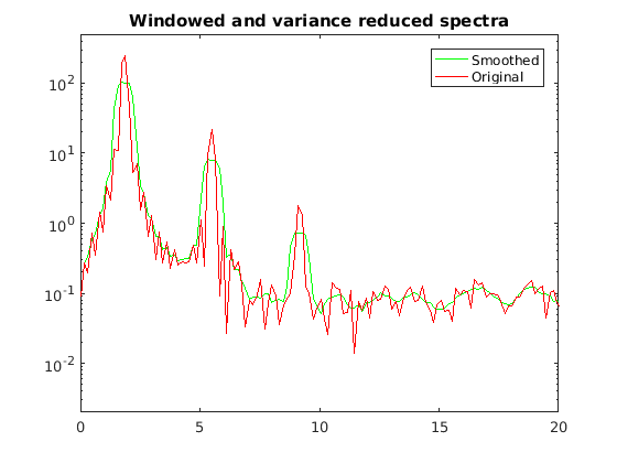
Note you don't quite get the same answer. Matlab's built in "pmtm" function is the engineering standard for spectra calculation.