1D Spectral Analysis

This script shows how to use the Fourier transform to look at the Power Spectral Density of a signal.

Make a grid and wavenumbers
Sample functions
Plots

close all;clear;

Make a grid and wavenumbers

N=1024;
L=20;

Make a grid that's one too long.

z=linspace(-1,1,N+1);

Truncate it.

z=z(1:end-1);

Make it the correct length for [-L,L].

x=z*L;
dx=x(2)-x(1);

The shortest wave number (equivalent to Nyquist frequency).

dk=pi/L;

This is Matlab's funny ordering for wavenumbers.

ksvec=zeros(size(x));
ksvec(1)=0;
ksvec(N/2+1)=0;
for ii=2:(N/2)
    ksvec(ii)=ii-1;
    ksvec(N/2+ii)=-N/2 + ii -1;
end
k=ksvec'*dk;
k2=k.*k;
ik=1i*k;

Sample functions

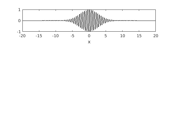
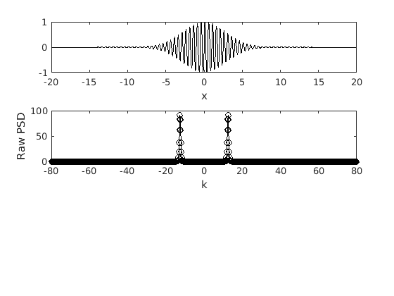
Gaussian packet.

f1=exp(-(x/4).^2).*sin(2*pi*x/0.5);

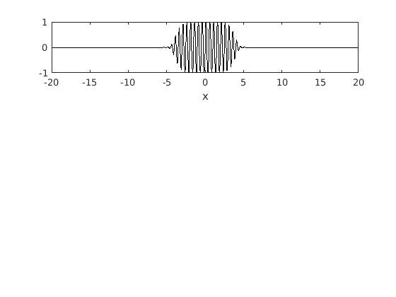
Super Gaussian packet.

f2=exp(-(x/4).^8).*sin(2*pi*x/0.5);

Two packets.

f3=exp(-((x-7.5)/4).^2).*sin(2*pi*x/0.5);
f3=f3+exp(-((x+7.5)/4).^2).*sin(2*pi*x/1);

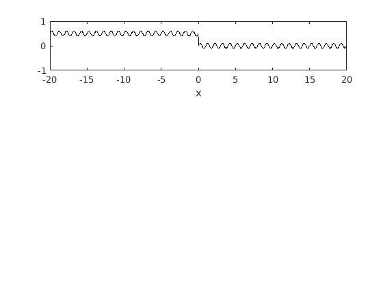
A function with a jump.

f4 = 0.1*sin(2*pi*x/1)-0.5.*heaviside(x)+0.5;

Plots

To calculate the PSD we take the absolute value of the Fast Fourier Transform (FFT) of the various functions.

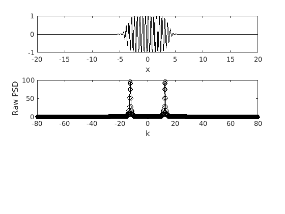
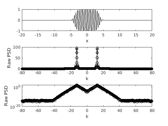
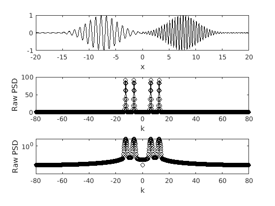
This subplot shows function.

figure(1)
subplot(3,1,1)
plot(x,f1,'-k')
xlabel('x')

Here we can see the spectra of the function.

subplot(3,1,2)
plot(k,abs(fft(f1)),'-ok')
xlabel('k')
ylabel('Raw PSD')
axis([-80 80 0 100])

We plot the spectra again, however we use a logarithmic scale for the power. This allows us to more clearly see the disparate scales.

subplot(3,1,3)
semilogy(k,abs(fft(f1)),'ok')
xlabel('k')
ylabel('Raw PSD')
axis([-80 80 1e-20 1e2])

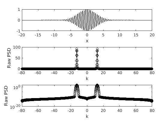
Using the semilog PSD we can easily see the spike at ~4 pi. We can also note that it is not a clean spike, but rather covers the wavenumbers around 4 pi as well. This is due to the Gaussian envelop used to create the packet. We can also note that the negative wavenumbers are a reflection of the positive ones and so they are not necessary.

The function.

figure(2)
subplot(3,1,1)
plot(x,f2,'-k')
xlabel('x')

The raw PSD.

subplot(3,1,2)
plot(k,abs(fft(f2)),'-ok')
xlabel('k')
ylabel('Raw PSD')
axis([-80 80 0 100])

The semilog PSD.

subplot(3,1,3)
semilogy(k,abs(fft(f2)),'ok')
xlabel('k')
ylabel('Raw PSD')
axis([-80 80 1e-20 1e2])

In this case we have a Super Gaussian packet which is to the power of 8 rather than the power of 2. This results in the edges of the packet becoming steeper. As a result, we can see that the spikes are much broader compared to those in the previous figure. Many more wavenumber are being activated in this case. This is because as you get closer to a vertical line (steeper) you require more and more wavenumbers.

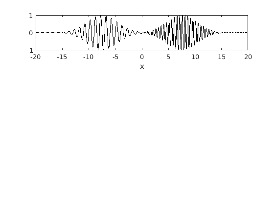
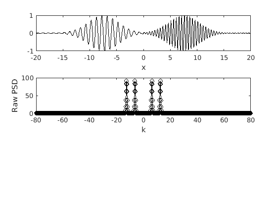
The function.

figure(3)
subplot(3,1,1)
plot(x,f3,'-k')
xlabel('x')

The raw PSD.

subplot(3,1,2)
plot(k,abs(fft(f3)),'-ok')
xlabel('k')
ylabel('Raw PSD')
axis([-80 80 0 100])

The semilog PSD.

subplot(3,1,3)
semilogy(k,abs(fft(f3)),'ok')
xlabel('k')
ylabel('Raw PSD')
axis([-80 80 1e-8 1e2])

In this case we have two packets with distinct wavenumbers occurring at different locations. We can clearly see the two spikes corresponding to the two wavenumbers.

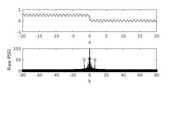
The function.

figure(4)
subplot(3,1,1)
plot(x,f4,'-k')
xlabel('x')

The raw PSD.

subplot(3,1,2)
plot(k,abs(fft(f4)),'-ok')
xlabel('k')
ylabel('Raw PSD')
axis([-80 80 0 100])

The semilog PSD.

subplot(3,1,3)
semilogy(k,abs(fft(f4)),'ok')
xlabel('k')
ylabel('Raw PSD')
axis([-80 80 1e-1 1e2])

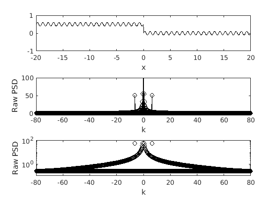
In this case we have a simple sine wave with an abrupt jump in it halfway through the domain. This vertical jump dramatically changes the spectrum. The first thing to note is the massively decreased axis, the minimum value is only ~10^0.5 which indicates that all wavenumbers have at least some power. We can also note that the there is a general increase in power for lower wavenumbers. This is all due to the well-known Gibbs phenomena.

1D Spectral Analysis

Contents

Make a grid and wavenumbers

Sample functions

Plots