Differentiation and Integration

This script is a tutorial on how to differentiate and integrate numerically. No fancy techniques are used and it is really an exercise in using the data structures learned in the first lesson.

Contents

Define parameters and set up the grid

numpts=1000;
L=10;

Set up the 1d grid.

xg=10*linspace(0,1,numpts+1); dx=xg(2)-xg(1);
xgm=0.5*(xg(2:numpts+1)+xg(1:numpts));
dxg=(xg(2:numpts+1)-xg(1:numpts));

Define the function

Define the function of interest, its derivative and integral (I used Maple).

myf=@(x) x.*(10-x).*sin(4*pi*x/L);
myfp=@(x) (10-x).*sin((2/5)*pi.*x)-x.*sin((2/5)*pi.*x)+(2/5)*x.*(10-x).*cos((2/5)*pi.*x)*pi;
myintf=@(x) (25/4)*(10*sin((2/5).*pi.*x)-4*x.*cos((2/5)*pi*x)*pi-(5/2)*(-(4/25)*pi^2*x.^2.*cos((2/5)*pi*x)+2*cos((2/5)*pi*x)+(4/5)*pi*x.*sin((2/5)*pi*x))/pi)/pi^2;
myg=@(x) 10*x-0.1*3*x.^2;
myintg=@(x) 5*x.^2-0.1*x.^3;

Get the function and the derivative on the grid.

fg=myf(xg);

For the derivative use the grid at the mid points.

fgp=myfp(xgm);

Finite Difference approximation

Now use a finite difference approximation that uses the info at the closest point on the right and the closest point on the left.

fpmethod1=(fg(2:end)-fg(1:end-1))./dxg;
figure(1)
clf
subplot(2,1,1)
plot(xgm,fgp,'b',xgm,fpmethod1,'ro')
xlabel('x')
ylabel('derivative')
subplot(2,1,2)
semilogy(xgm,abs(fpmethod1-fgp))
xlabel('x')
ylabel('error')

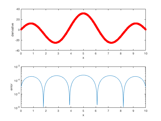
Try changing numpts to see how the error changes. The finite difference method in the above is of second order (you can check this from the Taylor series) but uses a different grid. We will talk about generating differentiation matrices in a different M-file but for now let's try to use interpolation onto the original grid to see how that effects the error.

fporig1=interp1(xgm,fpmethod1,xg,'linear');
fporig2=interp1(xgm,fpmethod1,xg,'pchip');
fporig3=interp1(xgm,fpmethod1,xg,'spline');

The moral of the story is that the built in spline interpolation is both quick and accurate.

fgp0=myfp(xg);
mxerrlin=max(abs(fporig1-fgp0))
mxerrcubic=max(abs(fporig2-fgp0))
mxerrspline=max(abs(fporig3-fgp0))

mxerrlin =

   9.5249e-04


mxerrcubic =

   9.5249e-04


mxerrspline =

   2.3813e-04

Integration

% Integration
gg=myg(xg);
% First order estimate of integral from the left and right Riemann sums.
myint1l=sum(gg(1:end-1))*dx;
myint1r=sum(gg(2:end))*dx;

Second order estimate of integral from the trapezoid rule. Notice that for not a lot of extra work we get a real improvement.

myint2=(0.5*gg(1)+sum(gg(2:end-1))+0.5*gg(end))*dx;
myinta=myintg(L)-myintg(0);
relerr1l=(myint1l-myinta)/myinta
relerr1r=(myint1r-myinta)/myinta
relerr2=(myint2-myinta)/myinta

relerr1l =

  -8.7513e-04


relerr1r =

   8.7487e-04


relerr2 =

  -1.2500e-07

Published with MATLAB® R2016b