Basic Matlab definitions and operations

This tutorial script shows the basic ways that Matlab can be used and some built-in operations.

A Calculator
Column and Row vectors
Matrix operations
Searching vectors
Function definition

A Calculator

From the start Matlab can be used as a basic calculator, for example:

5+2342
2354.3452*45345.23
234/23

ans =

        2347


ans =

   1.0676e+08


ans =

   10.1739

Column and Row vectors

Matlab's basic data structure is an array with the mathematical properties of a vector or matrix (an individual number is a scalar, or vector of length one). A vector can be created by using the "[]" symbols with spaces in between:

A=[ 1 2 3 4 5]

A =

     1     2     3     4     5

The default is to make a row vector. To make a column vector use the ";" symbol to separate:

B=[ 1; 2; 3; 4; 5]

Matrix operations

For another example, I define the number of rows and columns then I use the rand command to make up random vectors and matrices. Next I give examples of standard operations, including special Matlab operations.

numrows=5;
numcols=5;
myrowvec=rand(numrows,1);
mycolvec=rand(1,numcols);
mymatrix=rand(numrows,numcols);

Matrix multiplication right.

ans1=mymatrix*myrowvec

Matrix multiplication left.

ans2=mycolvec*mymatrix

ans2 =

    2.0461    2.3164    2.0875    1.2882    0.3671

Dot product method 1.

ans3=dot(myrowvec,mycolvec)

ans3 =

    1.8859

Dot product method 2.

ans3b=mycolvec*myrowvec

ans3b =

    1.8859

Outer product.

ans4=myrowvec*mycolvec

ans4 =

    0.0795    0.2269    0.4456    0.7801    0.7861
    0.0884    0.2523    0.4954    0.8673    0.8740
    0.0124    0.0354    0.0694    0.1216    0.1225
    0.0891    0.2544    0.4995    0.8746    0.8813
    0.0617    0.1761    0.3458    0.6055    0.6102

Transpose.

ans5=mymatrix'
myrowvec
ans6=myrowvec'

ans5 =

    0.1576    0.9706    0.9572    0.4854    0.8003
    0.1419    0.4218    0.9157    0.7922    0.9595
    0.6557    0.0357    0.8491    0.9340    0.6787
    0.7577    0.7431    0.3922    0.6555    0.1712
    0.7060    0.0318    0.2769    0.0462    0.0971


myrowvec =

    0.8147
    0.9058
    0.1270
    0.9134
    0.6324


ans6 =

    0.8147    0.9058    0.1270    0.9134    0.6324

Entry by entry multiplication.

ans7=myrowvec.*(2*ones(size(myrowvec)))
ans8=myrowvec.*mycolvec'

Searching vectors

Consider trying to find all the entries in a vector with a value larger than 0.5.

myrowvec2=rand(50000,1);

Time how long it takes.

tic
myind=zeros(size(myrowvec2));
for ii=1:50000
    if myrowvec2(ii)>0.5
        myind(ii)=1;
    end
end
time1=toc

time1 =

    0.0025

But Matlab is a vectorized language so for large vectors a much faster way to do this is to use the logical operations.

tic
myind2=(myrowvec2>0.5);
time2=toc

time2 =

   5.7922e-04

and it would be easy to have multiple ifs, say finding values between 0.5 and 0.75.

tic
myind3=((myrowvec2>0.5)&(myrowvec2<0.75));
time3=toc

time3 =

   7.8635e-04

The savings from vectorization become evident for large matrices. There is another related command that is sometimes useful.

myind=find(myrowvec2<0.5); % finds the indices of the entries in myrowvec2 that are less than a half.

IMPORTANT: IN GENERAL TRY TO AVOID FOR LOOPS IN MATLAB

Function definition

While Matlab has the means to create complex software structures involving functions I tend to prefer flat codes and for these inline function definitions are very useful. If you define your parameters before the function definition the functions will just use them all the time. This example is a traveling internal wave in a channel.

H=20; % total depth.
L=2*1e1; % wavelength.
k=2*pi/L; % wave number.
modenum=1; % mode number.
m=modenum*pi/H; % vertical wave number.
N0=2e-2; N02=N0^2; % buoyancy frequency and buoyancy frequency squared.
sigma=(N0*k*H)/sqrt(modenum^2*pi^2+k*H*k*H); % frequency.
myper=2*pi/sigma; % period.
amp=0.1;  % wave amplitude.

You use the th '@' symbol to define an anonymous function. Basically put @(variables) function_definition.

myf=@(x,z,t) amp*cos(k*x-sigma*t).*sin(m*z);
% To call the function we would just say:
wavenow=myf(0,H/2,0)

wavenow =

    0.1000

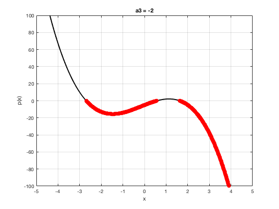
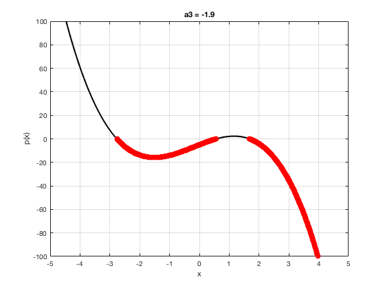
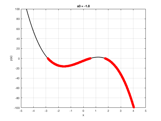
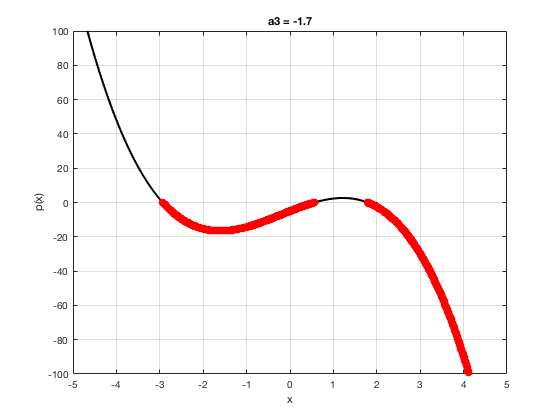
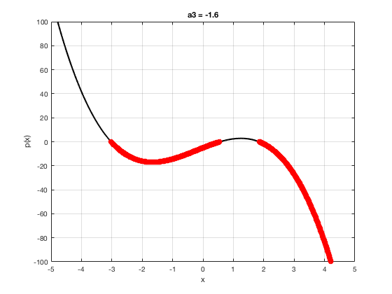
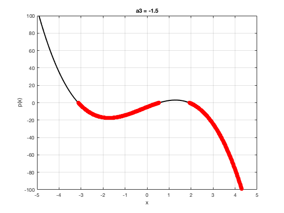
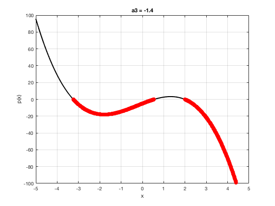
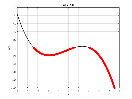
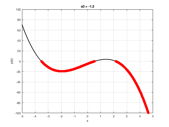
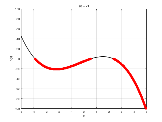
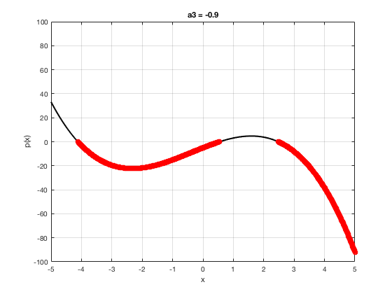
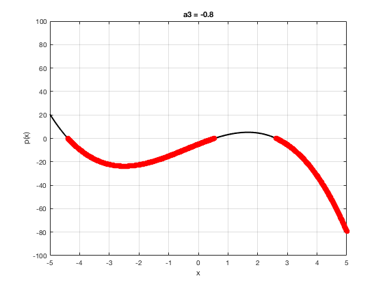
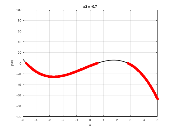
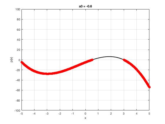
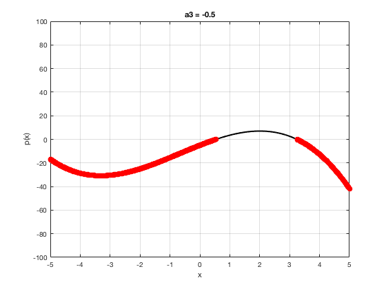
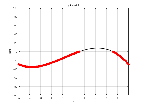
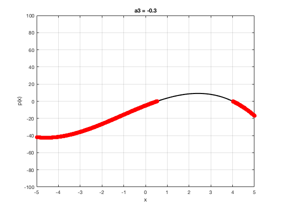
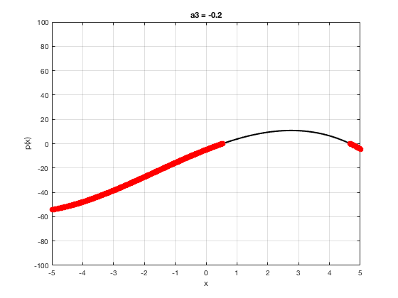
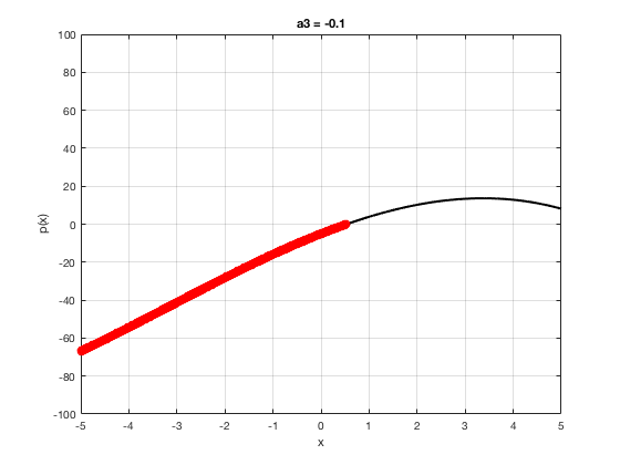
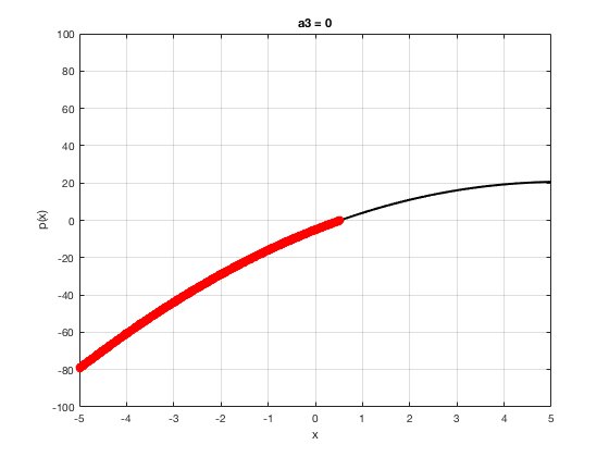
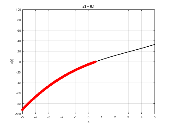
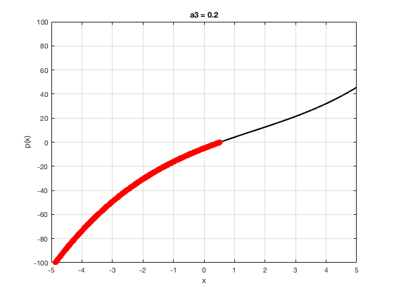
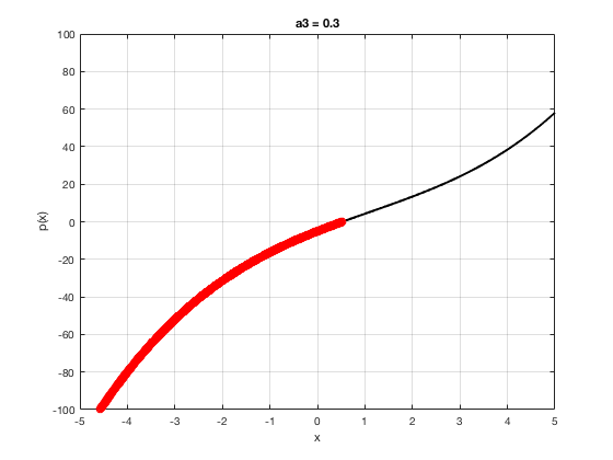
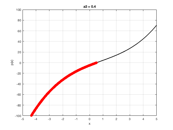
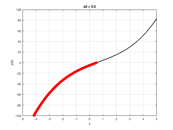
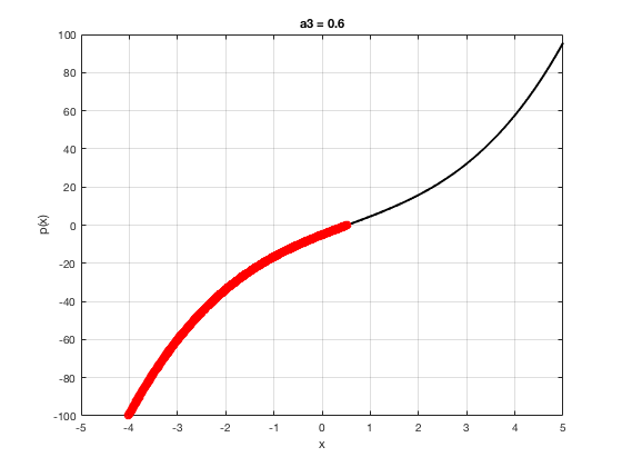
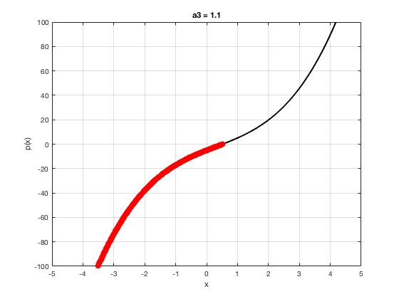
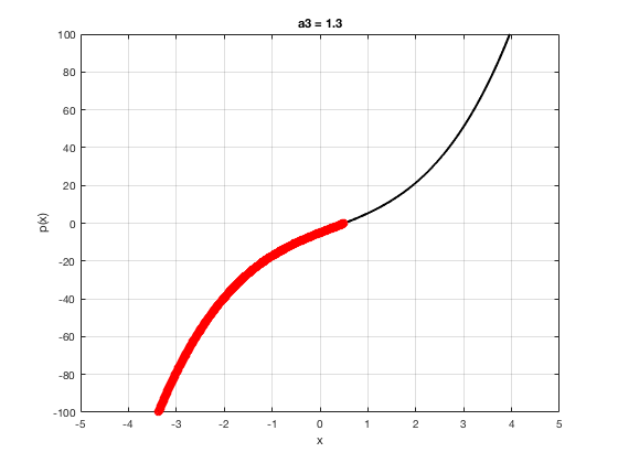
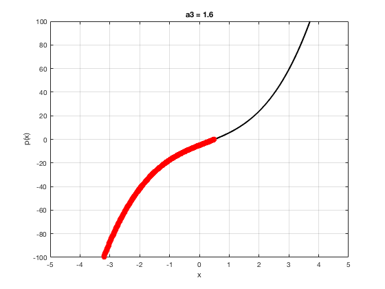
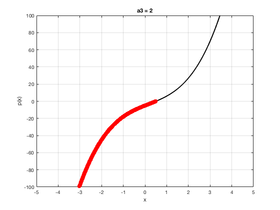
OK let's use all that to do something cool This loop makes a movie of the graph of a polynomial as the coefficient of the cubic term changes and marks the negative regions.

xg=linspace(-5,5,1001); % define a grid.
figure(1),clf % open a figure and clear it.
for a3=-2:0.1:2 % loop over the coefficient of x^3.

 myp=@(x) 0.001*x.^4+a3.*x.^3-x.^2+10*x-5;
 pg=myp(xg);
 myind=find(pg<0);
 clf
 plot(xg,pg,'k',xg(myind),pg(myind),'ro','linewidth',2)

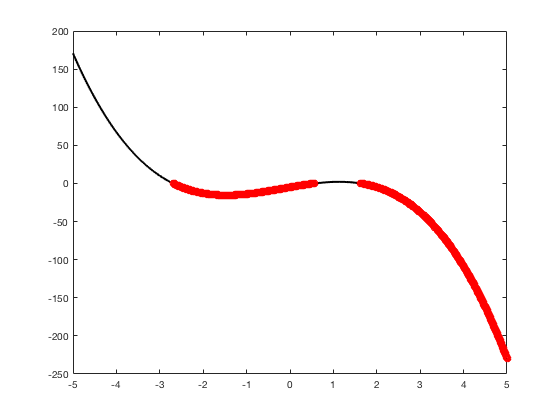
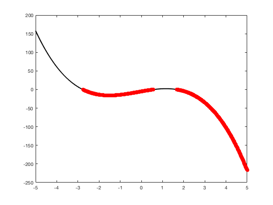
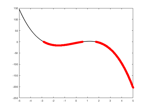
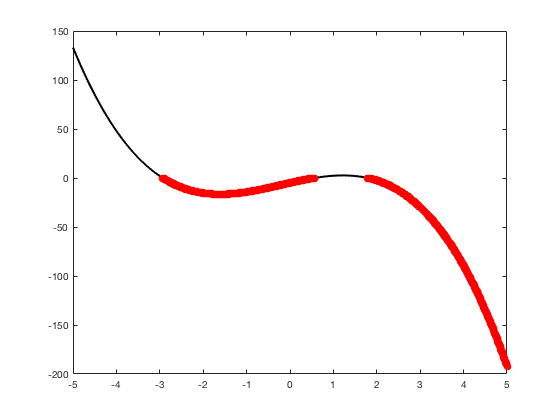
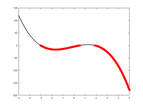
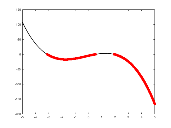
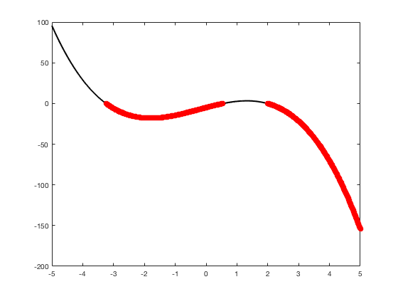
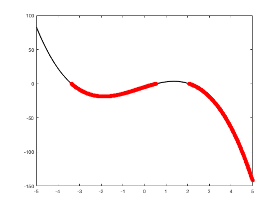
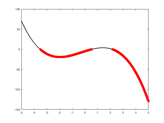
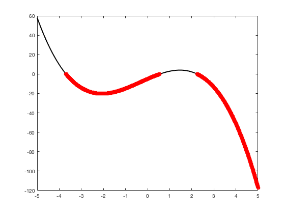
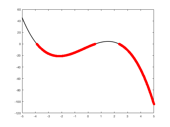
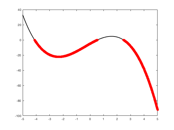
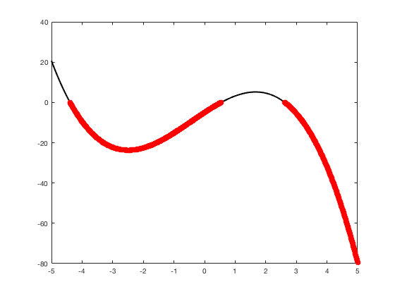
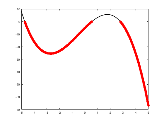
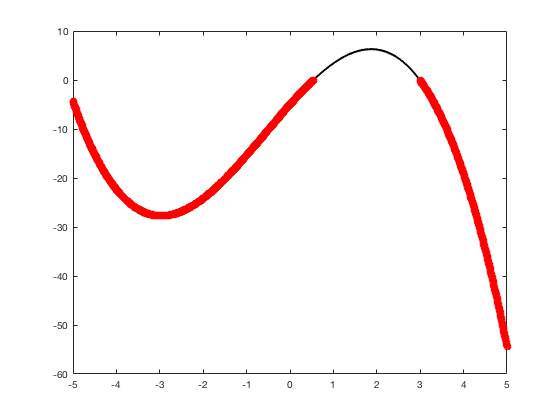
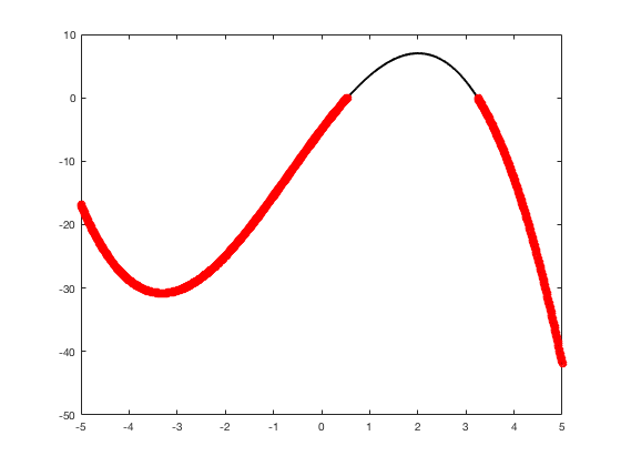
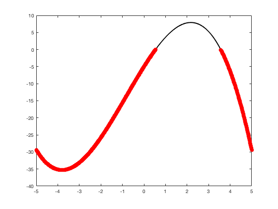
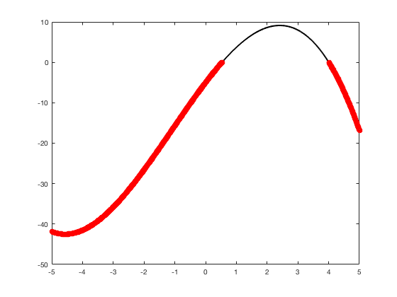
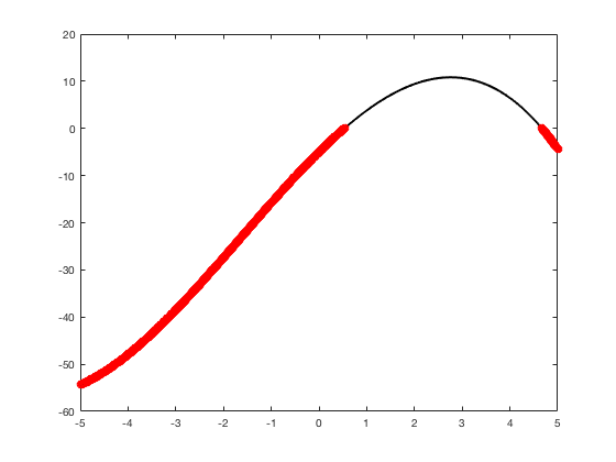
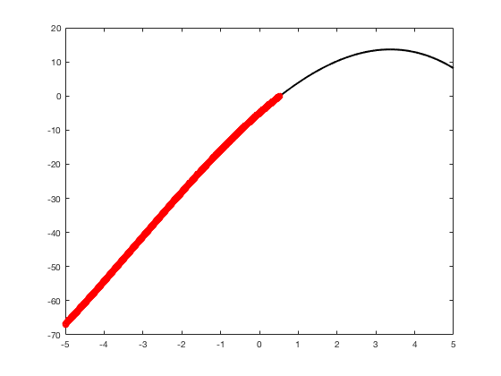
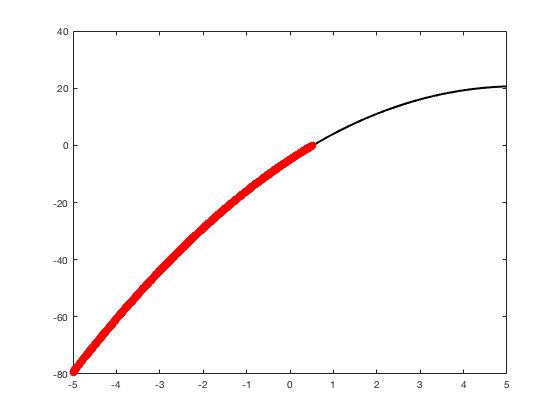
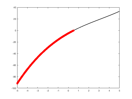
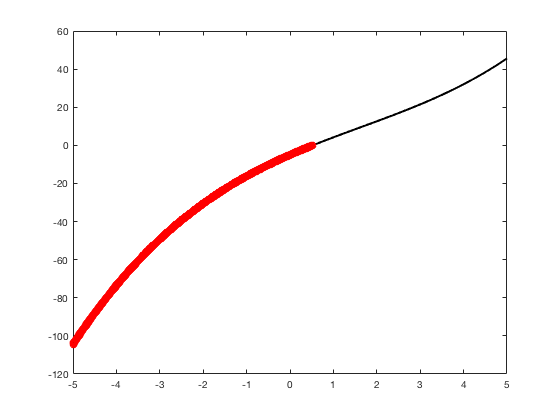
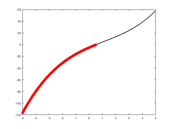
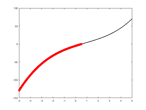
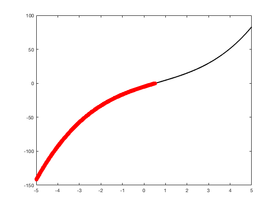
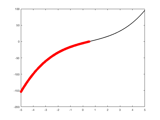
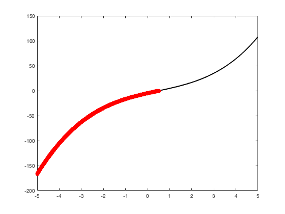
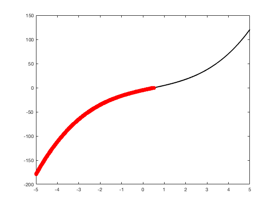
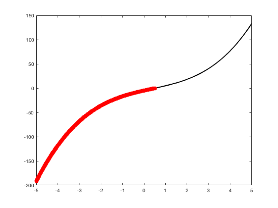
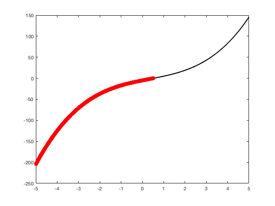
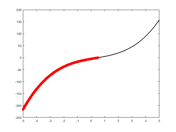
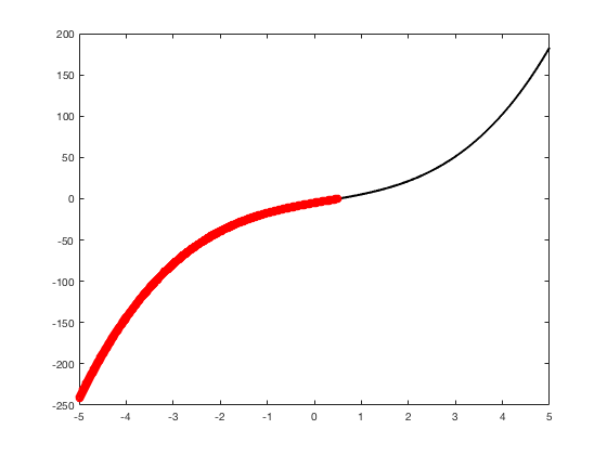
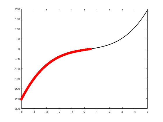
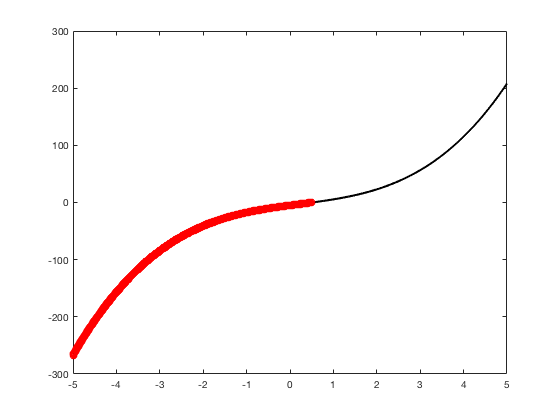
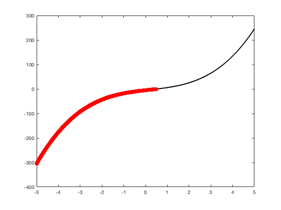
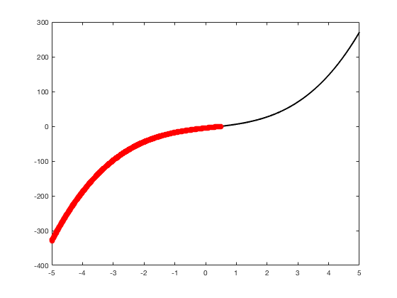
 xlabel('x') % label
 ylabel('p(x)') % label
 title(['a3 = ' num2str(a3,4)]) % title
 axis([-5 5 -100 100]) % fix the axis, [x_min x_max y_min y_max]
 grid on
 drawnow