Solving the Forced Damped Pendelum
The forced damped pendulum is one of the classic examples of a chaotic system. This script shows the various properties of a chaotic system. Please note that this script defines functions at the end, which is only supported by MATLAB 2016b or later. The equations of motion for this system are:
Contents

close all; clear
Initialization
omega_f = 2/3;
omega0 = 1;
q = 0.5;
F_d = 1.15;
We define the ICs.
phi0 = [0 0];
Solve the DE
Notice that the forcing function is a parameter that is passed to the DE function. This allows for it to be changed from this script.
tic
[ts, phis] = ode45(@(t,phi) func_dfpen(t, phi, omega0, q, F_d, omega_f, @(omega_f, t) cos(omega_f*t) ), [0 1000], phi0);
toc
Irregularity
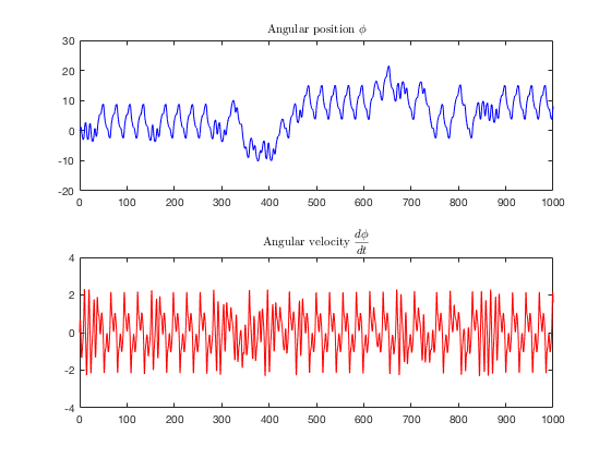
In this case we see that the position of the pendulum is not regular, There are periods where it appears to settle into regular oscillations, but they eventually stop and shift.
figure(1)
clf
subplot(2,1,1)
plot(ts,phis(:,1),'-b')
title('Angular position $$\phi$$','interpreter','latex')
subplot(2,1,2)
plot(ts,phis(:,2),'-r')
title('Angular velocity $$\frac{d\phi}{dt}$$','interpreter','latex')
Sensitivity to Initial Conditions
Now consider what happens when we VERY slightly change the initial conditions.
phi0=[1e-5 0];
tic
[ts2, phis2] = ode45(@(t,phi) func_dfpen(t, phi, omega0, q, F_d, omega_f, @(omega_f, t) cos(omega_f*t) ), [0 1000], phi0);
toc
figure(2)
clf
plot(ts,phis(:,1))
hold
plot(ts2,phis2(:,1))
legend('First IC','Second IC')
Elapsed time is 48.751648 seconds.
Current plot held
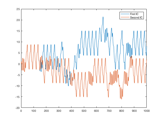
It is very clear that by ~150 the two cases become wildly different. This is with a very tiny difference, you can test that this still occurs with an even smaller initial difference.
Phase space
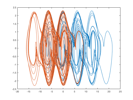
The differences between these cases can be very easily seen in the phase space plot. We can also see how chaotic an individual case is, oscillating around various fixed points randomly.
figure(3)
clf
plot(phis(:,1),phis(:,2))
hold on
plot(phis2(:,1),phis2(:,2))
The Damped Forced Pendulum
This function takes in time t, the angular position and angular velocity vector phi, the natural frequency omega0, the damping parameter q, the forcing magnitude F_d, the forcing frequency omega_f, and the forcing function force_fun.
function dphidt = func_dfpen(t, phi, omega0, q, F_f, omega_f, force_fun)
The ODE equations
These are constructed by converting the second order ODE to a system of first order DEs.
dphidt(1) = phi(2);
dphidt(2) = -omega0^2 * sin(phi(1)) - q*phi(2) + F_f*omega0^2*force_fun(omega_f,t);
dphidt=dphidt(:);
end
Elapsed time is 45.088572 seconds.