Solving a two box Lotka-Volterra system
The previous script was extremely simple and not particularly very useful. An extension of the original idea is that we have two predator-prey systems that are connected. An example of this could be two islands which are for the most part separate except for a small land bridge whereby some of the populations can interchange. In this case we would have the equations:


Please note that this script defines functions at the end, which is only supported by MATLAB 2016b or later.
Contents
close all;clear
Initialization
We now have different parameters for each box.
alpha = [2 2];
beta = [1/2 1];
delta = [1 2/3];
gamma = [4/3 1];
Correlation constants
New correlation constants for how the populations interchange.
First consider no interaction.
C_x = 0;
C_y = 0;
We define the ICs for both systems.
prey01 = 5;
pred01 = 10;
prey02 = 5;
pred02 = 1;
N0 = [prey01 pred01 prey02 pred02];
Use ODE45
Same form as the previous script, only with more parameters and a different function.
tic
[ts, Ns] = ode45(@(t,N) func_lotkavolterra2(t,N,alpha,beta,delta,gamma,C_x,C_y),[0 100],N0);
toc
Plot
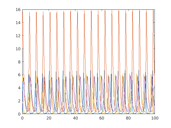
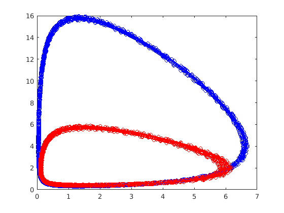
Results for the uncoupled case.
figure(1)
clf
plot(ts,Ns)
figure(2)
clf
plot(Ns(:,1),Ns(:,2),'-ob')
hold
plot(Ns(:,3),Ns(:,4),'-or')
Current plot held


Correlated case
Now consider a case where we allow for movement between the two boxes.
C_x = 1;
C_y = 1;

tic
[ts, Ns] = ode45(@(t,N) func_lotkavolterra2(t,N,alpha,beta,delta,gamma,C_x,C_y),[0 100],N0);
toc
Elapsed time is 57.687436 seconds.
Plot
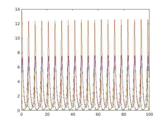
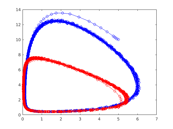
Results for the uncoupled case.
figure(1)
clf
plot(ts,Ns)
figure(2)
clf
plot(Ns(:,1),Ns(:,2),'-ob')
hold
plot(Ns(:,3),Ns(:,4),'-or')
Current plot held


This system will still form limit cycles, however the final state for each box is modified by the correlation values. Try testing different parameter values, especially when one box begins at a steady state.
The two box Lotka-Volterra equations
Two Lotka-Volterra boxes connected by a correlation term.
function dNdt = func_lotkavolterra2(t, N,alpha,beta,delta,gamma,C_x,C_y)
The ODE equations
The difference between this model and the single box model is the addition of the correlation terms which transfer population from the high population box to the low population one. The different parameters also allow for the boxes to have different steady states if there were no connection. The order of the populations is box 1: prey, predator, and box 2: prey predator.
dNdt(1) = alpha(1)*N(1)-beta(1)*N(1)*N(2)-C_x*(N(1)-N(3));
dNdt(2) = delta(1)*N(1)*N(2) - gamma(1)*N(2)-C_y*(N(2)-N(4));
dNdt(3) = alpha(2)*N(3)-beta(2)*N(3)*N(4)+C_x*(N(1)-N(3));
dNdt(4) = delta(2)*N(3)*N(4) - gamma(2)*N(4)+C_y*(N(2)-N(4));
dNdt = dNdt(:);
end
Elapsed time is 59.053217 seconds.