Annotating Figures

This script shows you how to annotate figures with arrows, lines and circles. It also shows you how the performance changes with increasing resolution.

N=128;
for cntr=0:5

    N=N*2
    x=linspace(-1,1,N);
    y=linspace(-1,1,N);
    [xx,yy]=meshgrid(x,y);
    myf=peaks(N);

N =

   256

N =

   512

N =

        1024

N =

        2048

N =

        4096

N =

        8192

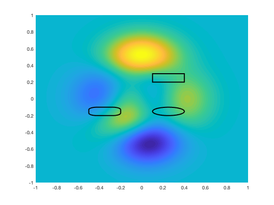
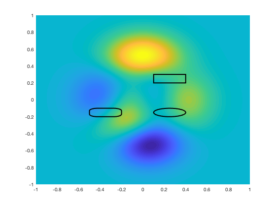
Some basic annotation sketches.

    tic
    figure(10*cntr+1)
    clf
    pcolor(xx,yy,myf),shading interp
    hold on
    rectangle('Position',[0.1 0.2 0.3 0.1],'LineWidth',2,'EdgeColor','k'); % rectangle
    rectangle('Position',[0.1 -0.2 0.3 0.1],'Curvature',[1 1],'LineWidth',2,'EdgeColor','k'); %ellipse
    rectangle('Position',[-0.5 -0.2 0.3 0.1],'Curvature',[0.5 0.6],'LineWidth',2,'EdgeColor','k') %rounded rectangle
    drawnow
    fig1time(cntr+1)=toc;

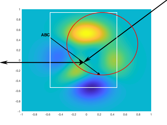
Now using the annotation command.

    tic
    figure(10*cntr+2)
    clf
    pcolor(xx,yy,myf),shading interp
    hold on
    ah=annotation('arrow',[1 .5],[1,.5],'Color','k','LineWidth',3,'HeadWidth',15,'HeadLength',25);
    a2=annotation('doublearrow',[0 .5],[0.5 0.5],'Color','k','LineWidth',3,'Head1Width',15,'Head1Length',25,'Head2Width',25,'Head2Length',15);
    th=annotation('textarrow',[.3,.6],[.7,.4],'String','ABC','LineWidth',2,'FontWeight','bold','FontSize',14);
    rh=annotation('rectangle',[.3 .3 .4 .6],'Color','w','LineWidth',2);
    eh=annotation('ellipse',[.4 .4 .425 .5],'Color','r','LineWidth',2);
    drawnow
    fig2time(cntr+1)=toc;

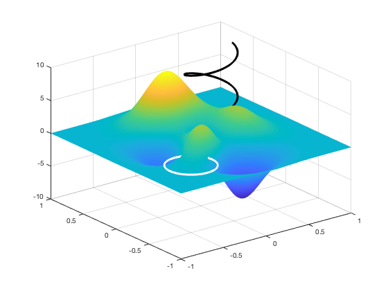
Putting annotations on a 3D plot.

    tic
    figure(10*cntr+3)
    clf
    surf(xx,yy,myf),shading interp
    hold on
    mys=linspace(0,6*pi,1000);
    myx=0.5+0.25*cos(mys);
    myy=0.5+0.25*sin(mys);
    myz=10*(mys-3*pi)/(3*pi);
    plot3(myx,myy,myz,'k-','LineWidth',3)
    mys=linspace(0,2*pi,1000);
    myx=-0.5+0.25*cos(mys);
    myy=-0.5+0.25*sin(mys);
    myz=0.25*ones(size(mys));
    plot3(myx,myy,myz,'w-','LineWidth',3)
    drawnow
    fig3time(cntr+1)=toc;

end

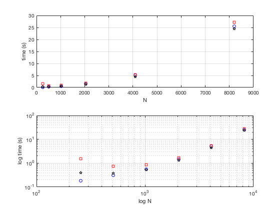
Based on the timing here after a resolution of 1024 there is a quadratic growth in elapsed time.

figure(5)
clf
myNs=256*2.^(0:5);
subplot(2,1,1)
plot(myNs,fig1time,'bo',myNs,fig2time,'rs',myNs,fig3time,'kp')
xlabel('N')
ylabel('time (s)')
grid on
subplot(2,1,2)
loglog(myNs,fig1time,'bo',myNs,fig2time,'rs',myNs,fig3time,'kp')
xlabel('log N')
ylabel('log time (s)')
grid on

Published with MATLAB® R2017a