Matlab 3D Graphics

This is a tutorial on the 3D graphics capabilities in Matlab.

Contents

Create data

We begin by creating some sample 3D data.

x=linspace(-1,1,256); % Create 1D grids.
y=linspace(-2,2,128);
z=linspace(-5,5,384);
[xxx,yyy,zzz]=meshgrid(x,y,z); % Combine to make 3D grid.
myf=sin(pi*xxx.*yyy).*(yyy.^2-3*xxx.*yyy.*zzz);
xg=xxx;
yg=yyy;
zg=zzz;
fg=myf;

Isosurface plot

figure(1)
clf
tic
% isosurface creates a 3D contour at the specified value (in this case 15).
p1=patch(isosurface(xg,yg,zg,fg,15));

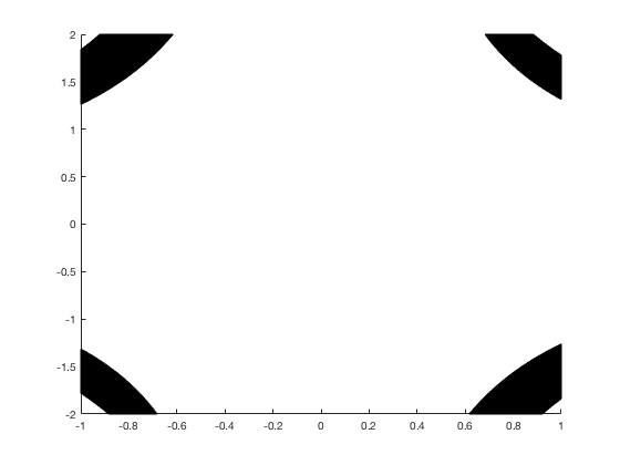
Using the "FaceColor" property you can change the color of the contour. These are defined using the RGB values, some common colors are: [0 0 1] Blue [1 0 0] Red [0 1 0] Green [1 1 0] Yellow [1 1 1] White [0 0 0] Black

p1.FaceColor = [0.95 0.05 0.05];

The "EdgeColor" property color sets the color of the edges of the surface. To remove any color from the edges, set this to none.

p1.EdgeColor = 'none';

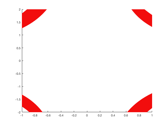
With the "FaceAlpha" property you can change the opacity of the contour.

p1.FaceAlpha = 0.55;

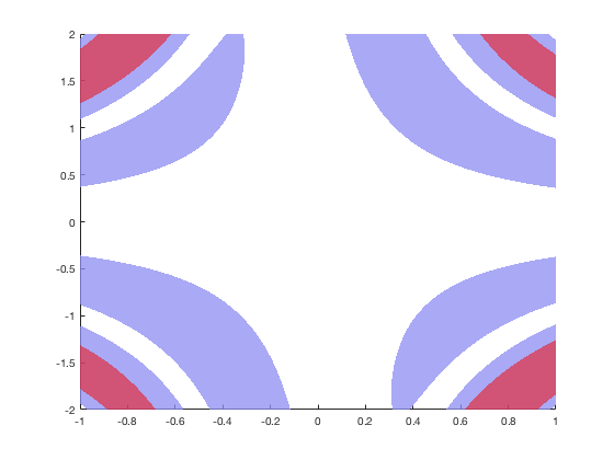
If you want to keep adding plots to the current figure you need to "hold" the figure.

hold on
p2=patch(isosurface(xg,yg,zg,fg,5));
p2.FaceColor = [0.55 0.55 0.95];
p2.EdgeColor = 'none';
p2.FaceAlpha = 0.75;

The view command changes the angle of the viewpoint for your figure. The first number is the azimuthal angle in degrees away from the negative y axis, and the second number is the angle of elevation away from the xy-plane. To see a diagram showing the angles go to: https://www.mathworks.com/help/matlab/ref/view.html?searchHighlight=view&s_tid=doc_srchtitle.

view([120 30])
grid on

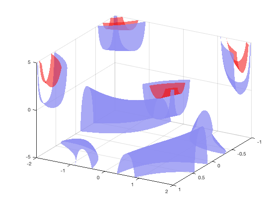
With 3D graphics you can control the "light" which creates shadows to create a more "realistic" figure. The "camlight" function specifies a light in the camera "view" coordinates (azimuthal and elevation). Every invocation will create a new light.

camlight(-45,0.1)
camlight(45,30)

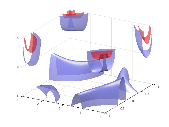
Since the x, y, and z grids are different lengths we can use the "daspect" command to change their aspect ratio so that the axes appear to be equal lengths.

daspect([1 2 5])
toc

Elapsed time is 6.048523 seconds.

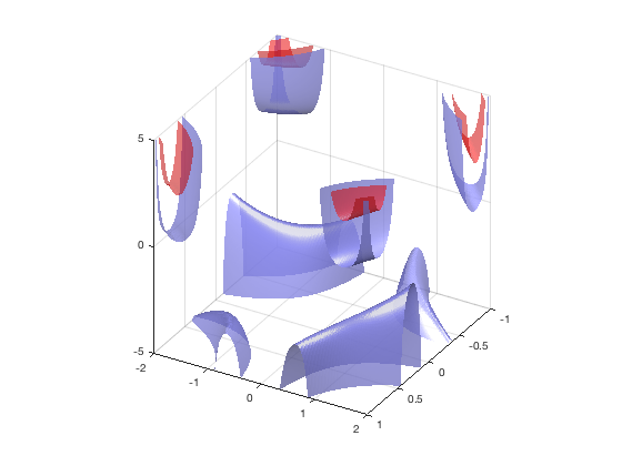
Changing the viewer size

If we wanted to make all the axis lengths appear their actual sizes you change the daspect to [1 1 1].

figure(2)
clf
tic
p1=patch(isosurface(xg,yg,zg,fg,15));
p1.FaceColor = [0.95 0.05 0.05];
p1.EdgeColor = 'none';
p1.FaceAlpha = 0.55;
hold on
p2=patch(isosurface(xg,yg,zg,fg,5));
p2.FaceColor = [0.55 0.55 0.95];
p2.EdgeColor = 'none';
p2.FaceAlpha = 0.75;
view([120 30])
grid on
camlight(-45,0.1)
camlight(45,30)
daspect([1 1 1])

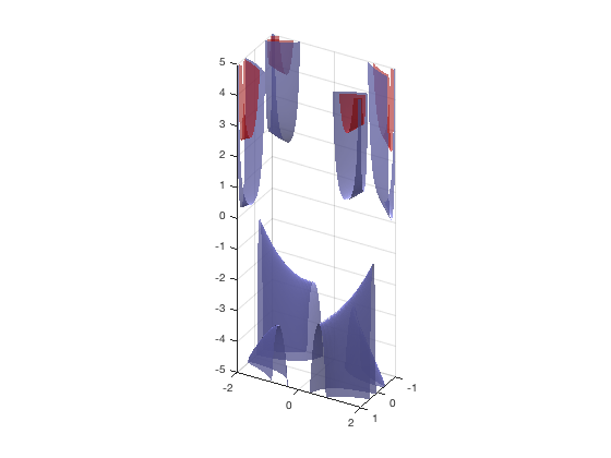
Where the daspect([1 1 1]) specifies that all axis should be the same size.

Notes

Some other plotting functions which work in 3D are: surf quiver streamline To see the full selection of functions please go to: https://www.mathworks.com/help/matlab/2-and-3d-plots.html

Published with MATLAB® R2016b