Parallel and GPU computing

Matlab has made it extremely easy to use parallel and GPU computing. For parallel computing the most direct and easiest way to implement it is through the "parfor" command.

Contents

Parallel Computing

To initialize the set of parallel "workers" that will be used, use the "parpool" command.

parpool

Starting parallel pool (parpool) using the 'local' profile ... connected to 4 workers.

ans = 

 Pool with properties: 

            Connected: true
           NumWorkers: 4
              Cluster: local
        AttachedFiles: {}
          IdleTimeout: 30 minute(s) (30 minutes remaining)
          SpmdEnabled: true

This will use the default cluster profile, and for most personal computers this will work fine. However, for other types of systems you can also use "parpool" to configure the workers how you like.

If you have a range of consecutive, finite integers over which you are performing a "for" loop, "parfor" will most likely be faster. Consider the following loop.

n=500;
ranksSingle=zeros(1,n);
tic
for ind=1:n
    ranksSingle(ind) = rank(magic(ind));
end
toc

Elapsed time is 13.223955 seconds.

Now consider:

ranks=zeros(1,n);
tic
parfor ind=1:n
    ranks(ind) = rank(magic(ind));
end
toc

Elapsed time is 5.658752 seconds.

Depending on the speed of your processors and the number of cores your computer has this will either be substantially or somewhat faster than the serial "for". In most cases this is all the parallelization you will need to see significant speed up in your code.

If you are working on a distributed cluster or are using a particular Matlab Toolbox please visit: https://www.mathworks.com/help/distcomp/getting-started-with-parallel-computing-toolbox.html Here you can find information and examples for using the other parallel features.

% Aaron's Laptop:
% 5.88s 1 worker
% 2.783 4 workers

close all;clear;

GPU Computing

If you have many small tasks which do not require much memory (running an ensemble of stochastic simulations is the classic example) then GPU computing can offer immense speed ups.

The Graphical Processing Unit (GPU) is a dedicated piece of hardware that is primarily used when displaying or rendering graphics. It has a different architecture than the standard Central Processing Unit (CPU) that most computing is done with. Specifically, it has a huge number of cores (usually more than 1000) but relatively low amounts of memory which is shared between cores. When displaying or rendering graphics many vector operations must be performed. As graphics became more and more important a separate unit was developed to take the load off of the CPU.

What is key to remember when working with GPU computing is that the GPU is a separate unit with its own memory which is separate from the CPU. To create an array on the GPU you use the "gpuArray" class which has many of the standard array functions, but creates it on the GPU.

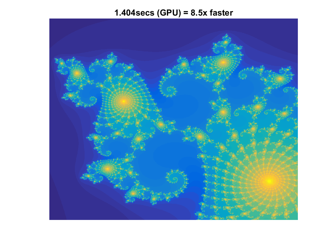
Here we will be following the example on: https://www.mathworks.com/help/distcomp/examples/illustrating-three-approaches-to-gpu-computing-the-mandelbrot-set.html This renders a visualization of the Mandelbrot Set. This example is without using the GPU:

maxIterations = 500;
gridSize = 1000;
xlim = [-0.748766713922161, -0.748766707771757];
ylim = [ 0.123640844894862,  0.123640851045266];

Setup

t = tic();
x = linspace( xlim(1), xlim(2), gridSize );
y = linspace( ylim(1), ylim(2), gridSize );
[xGrid,yGrid] = meshgrid( x, y );
z0 = xGrid + 1i*yGrid;
count = ones( size(z0) );

Calculate

z = z0;
for n = 0:maxIterations
    z = z.*z + z0;
    inside = abs( z )<=2;
    count = count + inside;
end
count = log( count );

Show

cpuTime = toc( t );
figure(1)
imagesc( x, y, count );
axis off
title( sprintf( '%1.2fsecs (without GPU)', cpuTime ) );

We now begin the GPU version.

Setup

t = tic();
% We use the gpuArray.linspace to create an equispaced grid IN THE GPU
% MEMORY.
x = gpuArray.linspace( xlim(1), xlim(2), gridSize );
y = gpuArray.linspace( ylim(1), ylim(2), gridSize );
[xGrid,yGrid] = meshgrid( x, y );
z0 = complex( xGrid, yGrid );

This is another way of initializing an array on the GPU.

count = ones( size(z0), 'gpuArray' );

Now we can work in the standard way with these objects.

Calculate

z = z0;
for n = 0:maxIterations
    z = z.*z + z0;
    inside = abs( z )<=2;
    count = count + inside;
end
count = log( count );

Since the variable "count" was initialized on the GPU we don't actually have the computed data in the processor (and hence Matlab workspace) memory. To bring it back to the CPU we use the "gather" command.

count = gather( count ); % Fetch the data back from the GPU.
GPUTime = toc( t );
figure(2)
imagesc( x, y, count )
axis off
title( sprintf( '%1.3fsecs (GPU) = %1.1fx faster', ...
    GPUTime, cpuTime/GPUTime ) )

% Aaron's Laptop (GTX 860M)
% 19.07s CPU
% 2.256s GPU
delete(gcp('nocreate'))

Parallel pool using the 'local' profile is shutting down.

Published with MATLAB® R2016a