Sturm-Liouville eigenvalue problem solver including projections
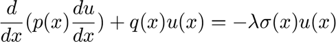
This script solves the classical Sturm-Liouville problem. This problem appears throughout applied mathematics and is similar to the traditional eigenvalue problem from linear algebra. However rather than a matrix we now have an operator and the variables are functions. We then project a function onto the basis formed by the eigenfunctions. The equations are:

The inner product is 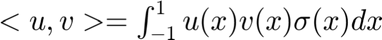 .
.
Contents
clear all
format long, format compact
Number of points and the derivative and integration material.
N=50;
[D,x]=cheb(N); D2=D^2; % Differentiation matrices.
[xi wt]=clencurt(N); % Integration coefficients.
Note the computational domain is [-1,1]
Define the various functions.
numdx=1e-8;
myp=@(x) 1+exp(-(x/0.2).^2);
mypx=@(x) (myp(x+numdx)-myp(x-numdx))/(2*numdx);
myq=@(x) x;
mysig=@(x) 1+0.5*sin(x*pi);
Build the operators.
myoplh=diag(myp(x))*D2+diag(mypx(x))*D+diag(myq(x));
myoprh=diag(mysig(x));
The boundary conditions are u=0 so just strip off the first and last row and column.
myoprh=myoprh(2:end-1,2:end-1);
myoplh=myoplh(2:end-1,2:end-1);
Solve the eigenvalue problem and sort the eigenvalues.
[myphis0 mylams0]=eig(myoplh,myoprh);
[mylams mylamsi]=sort(diag(mylams0),'descend');
Set the number of modes you wish to consider.
num_modes=20;
modesu=zeros(N+1,num_modes);
modesu(2:N,:)=myphis0(:,mylamsi(1:num_modes));
modese=zeros(size(modesu));
Calculate Modes
for k=1:num_modes
unow=modesu(:,k);
Normalize using the inner product.
    normalizationu(k)=sqrt(sum(wt'.*unow.^2.*mysig(x)));
    modesu(:,k)=unow/normalizationu(k);
Notice the way the Clenshaw Curtis weights come in.
end
Figure 1
figure(1)
clf
set(gcf,'DefaultLineLineWidth',2,'DefaultTextFontSize',12,...
    'DefaultTextFontWeight','bold','DefaultAxesFontSize',12,...
    'DefaultAxesFontWeight','bold');
plot(mylams(1:20),'bo')
xlabel('mode number')
ylabel('frequency')
grid on
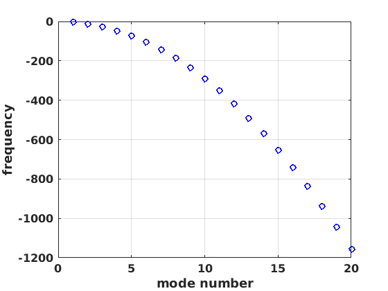
Figure 2
figure(2)
clf
set(gcf,'DefaultLineLineWidth',2,'DefaultTextFontSize',12,...
    'DefaultTextFontWeight','bold','DefaultAxesFontSize',12,...
    'DefaultAxesFontWeight','bold');
plot(x,myp(x),'k-',x,myq(x),'b-',x,mysig(x),'r')
xlabel('x')
xlabel('Sturm Liouville functions')
legend('p(x)','q(x)','\sigma(x)')
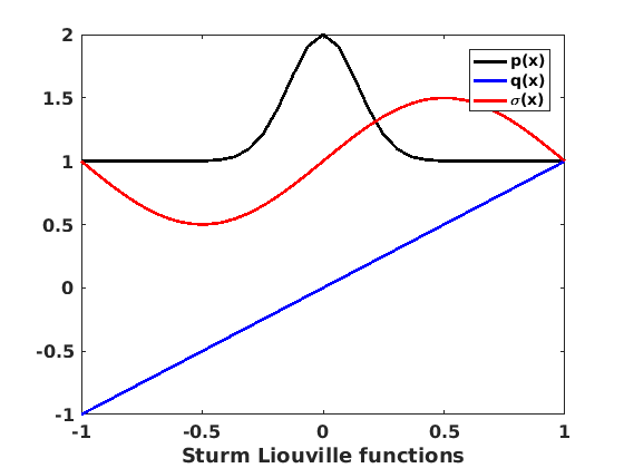
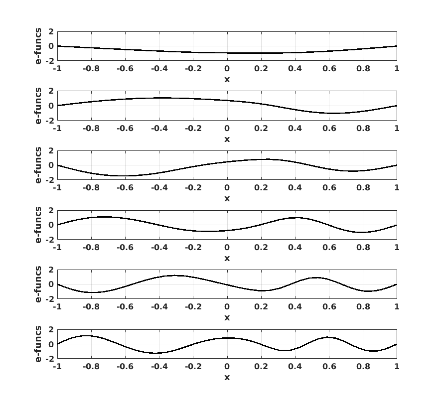
Figure 3
figure(3)
clf
set(gcf,'DefaultLineLineWidth',2,'DefaultTextFontSize',12,...
    'DefaultTextFontWeight','bold','DefaultAxesFontSize',12,...
    'DefaultAxesFontWeight','bold');
for modei=1:6
    subplot(6,1,modei)
    plot(x,modesu(:,modei),'k-')
    xlabel('x')
    ylabel('e-funcs')
    grid on
    axis([-1 1 -2 2])
end
Projections
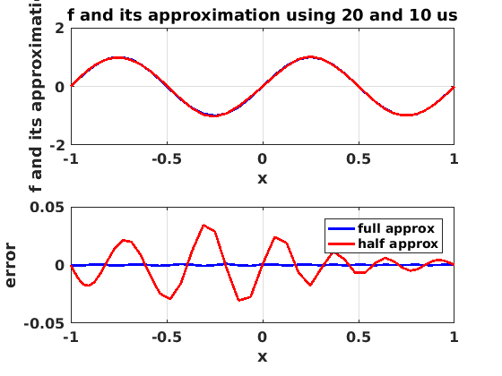
Now for some projections. First choose the function to project. Anything that satisfies the BCs is OK.
f=sin(2*pi*x);
myapp=zeros(size(f));
for k=1:num_modes/2
    phinow=modesu(:,k);
    coeff(k)=sum(wt'.*phinow.*f.*mysig(x));
    myapp=myapp+coeff(k)*phinow;
end
myapphalf=myapp;
for k=(num_modes/2+1):num_modes
    phinow=modesu(:,k);
    coeff(k)=sum(wt'.*phinow.*f.*mysig(x));
    myapp=myapp+coeff(k)*phinow;
end
Figure 4
figure(4)
clf
set(gcf,'DefaultLineLineWidth',2,'DefaultTextFontSize',12,...
    'DefaultTextFontWeight','bold','DefaultAxesFontSize',12,...
    'DefaultAxesFontWeight','bold');
subplot(2,1,1)
plot(x,f,'k',x,myapp,'b',x,myapphalf,'r')
xlabel('x')
ylabel('f and its approximation')
grid on
title(['f and its approximation using ' int2str(num_modes) ' and ' int2str(num_modes/2) ' us'])
subplot(2,1,2)
plot(x,f-myapp,'b',x,f-myapphalf,'r')
legend('full approx','half approx')
grid on
xlabel('x')
ylabel('error')