FFT based method for advection type models (Burgers)

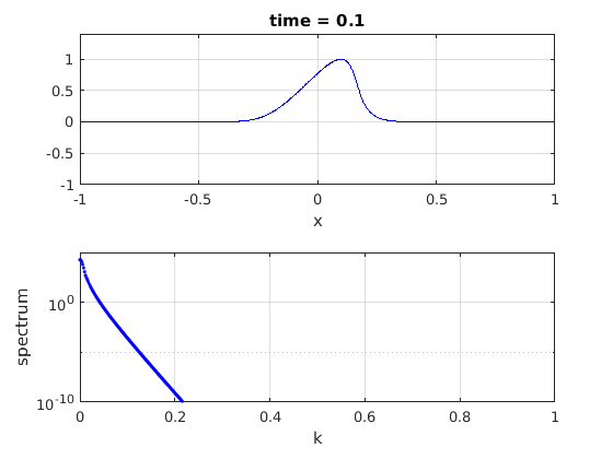
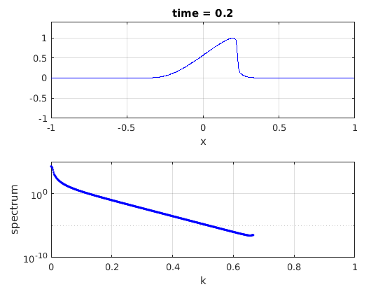
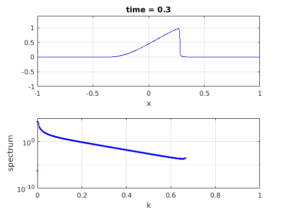
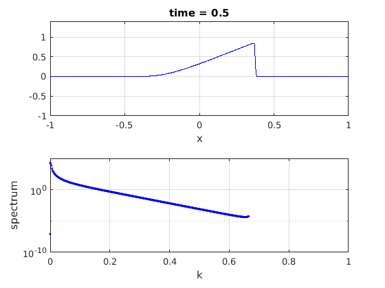
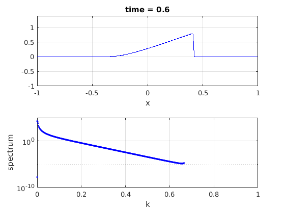
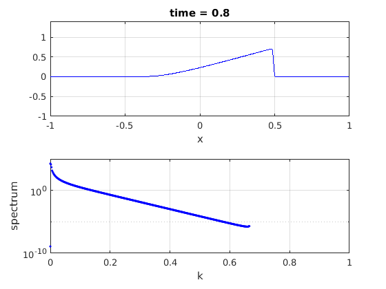
This script solves the Burgers equation using spectral methods. The waves will eventually steepen and form a shock which is a problem for spectral methods. This model has viscosity which can tame the shock formation however many times this is not enough. To fix this we can use spectral filters which help stop the build up of high wavenumbers (when it steepens to a shock). There are multiple different filters provided in the script. Currently it uses Boyd's 2/3 filter however you can easily modify the code to use a different one.

Contents

clear all; close

Parameters

Define physical parameters for the model.

nu = 1e-3;

Define a spatial grid.

xmin = -1;
xmax = 1;
N = 2^10;
x = linspace(xmin,xmax,N+1);
x = x(1:N);
dx = x(2)-x(1);
L = xmax - xmin;

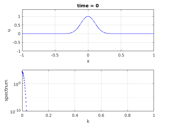
Make initial condition.

u_amp = 1;
sig = 0.15*xmax;
u = u_amp*exp(-(x/sig).^2);
u0 = u;

Time step and number of steps.

t = 0;          % initial time
t_f = 1;      % final time
t_plot = 0.1;  % plot interval
dt = 1e-3;      % time step

Total steps and plot steps.

N_stps = round(t_f/dt);
N_plot = round(t_plot/dt);

Wave numbers.

dk = 2*pi/L;
ks = [0:N/2-1 0 -N/2+1:-1]*dk;
ks2 = ks.*ks;
kmax = max(abs(ks));

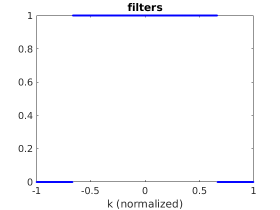
Filters

Define specific filters: Boyd 2/3 filter.

f_step = @(kc,k) 1.*(abs(k)<kc) + 0.*(abs(k)>=kc);
f_23 = @(k) f_step(2/3, k);

Gaussian filter.

f_gauss = @(a,b,kc,k) 1.*(abs(k)<=kc) + min(1, exp(-a*(abs(k)-kc).^b./(1-kc).^b)).*(abs(k)>kc);

Hyperviscosity.

f_hyper = @(a,b,k) exp(-a*abs(k).^b);

Bump filters.

f_bump  = @(a,b,kc,k) 1.*(abs(k)<=kc) + min(1, exp(a*(1-1./(1-((abs(k)-kc)./(1-kc)).^b)))).*(abs(k)>kc);
f_bump2 = @(a,b,k1,k2,k) 1.*(abs(k)<=k1) ...
          + min(1, exp(a*(1-1./(1-((abs(k)-k1)./(k2-k1)).^b)))).*(abs(k)>k1 & abs(k)<k2) ...
          + 0.*(abs(k)>=k2);

Parameters.

filt_alpha = 0.2;
filt_beta = 4;
kcut = 0.5*kmax;
u_filter = f_23(ks/kmax);

Ploting

Plot initial conditions.

figure(2)
clf
subplot(2,1,1)
plot(x,u,'b-')
grid on
xlabel('x');
ylabel('u');
title(['time = ' num2str(t,2)]);
axis([xmin xmax -max(abs(u0)) 1.4*max(abs(u0))])
subplot(2,1,2)
uf = fft(u);
spec1 = uf.*conj(uf);
plot(fftshift(ks)/kmax,abs(fftshift(spec1)),'b.')
xlabel('k');
ylabel('spectrum');
grid on
axis([0 1 1e-10-eps 1e5])
set(gca,'yscale','log')
drawnow

Plot the filter.

figure(1)
clf
plot(ks/max(ks),u_filter,'b.')
title('filters')
xlabel('k (normalized)')

Main Loop

LHS of implicit formulation.

lhopu = 1 + dt*ks2*nu;

Euler time stepping

for ii=1:N_stps

    t = t+dt;

Compute the nonlinear terms (these are treated explicitly).

    uux = u.*ifft(i*ks.*fft(u));
    uxx = ifft(-ks2.*fft(u));

Now in the transformed domain treat the diffusion implicitly.

    rhs = u - dt*uux + dt*nu*uxx;
    uincr = real(ifft(u_filter.*(fft(rhs))));
    u = uincr(1:N);
    if sum(isnan(u)) > 0
        disp(['simulation broke at t=',num2str(t)])
        return
    end
    if mod(ii,N_plot) == 0

Plot

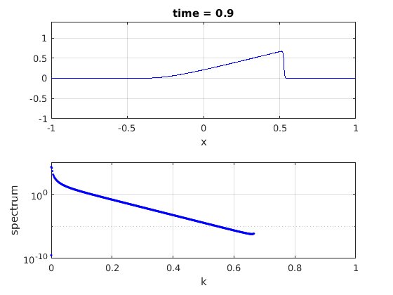
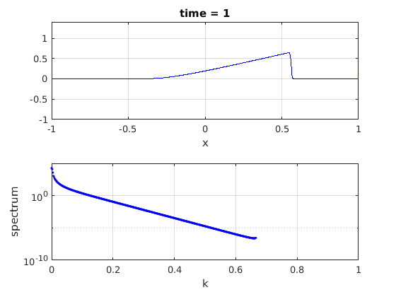
Update the plots.

        figure(2)
        clf
        subplot(2,1,1)
        plot(x,u,'b-')
        grid on
        xlabel('x');
        title(['time = ' num2str(t,3)]);
        axis([xmin xmax -max(max(u0)) 1.4*max(max(u0))])
        subplot(2,1,2)
        uf = fft(u);
        spec1 = uf.*conj(uf);
        plot(fftshift(ks)/kmax,abs(fftshift(spec1)),'b.')
        xlabel('k');
        ylabel('spectrum');
        grid on
        axis([0 1 1e-10-eps 1e5])
        set(gca,'yscale','log')
        drawnow

    end

end

Published with MATLAB® R2016b